In today’s tutorial, I’ll provide some techniques and tips on how to deal with common problems caused by DAX weekly granularity in time intelligence calculations. You can watch the full video of this tutorial at the bottom of this blog.
I recently did a tutorial on obtaining Previous Week Values in Power BI. Since then, I’ve got several questions related to time intelligence and particularly related to DAX weekly values. That’s not surprising because weeks are really the most poorly behaved granularity in the time intelligence sphere.
In the case of months, you’ve always got 12 months in a year. In the case of quarters, you’ve always got four quarters. Weeks are different because there are seven days in a week and 52 weeks in a year – that’s 364 days. So, you’ve got that extra day hanging out there. In Leap years, you’ve got two extra days.
So, that actually ends up in some years, based on the numbering scheme for the ISO week number, to have sometimes 52 weeks, sometimes 53 weeks. Week 53 is the one that’s going to cause the most problems.
Time Intelligence Issues Of A DAX Weekly Calculation
In this example, I’m using Total Spot Price. With totals, it’s easier to visualize and talk about.
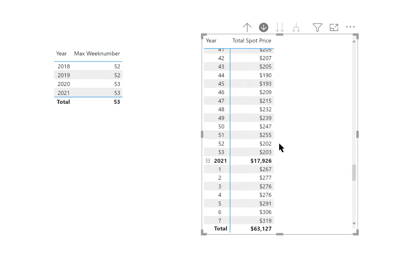
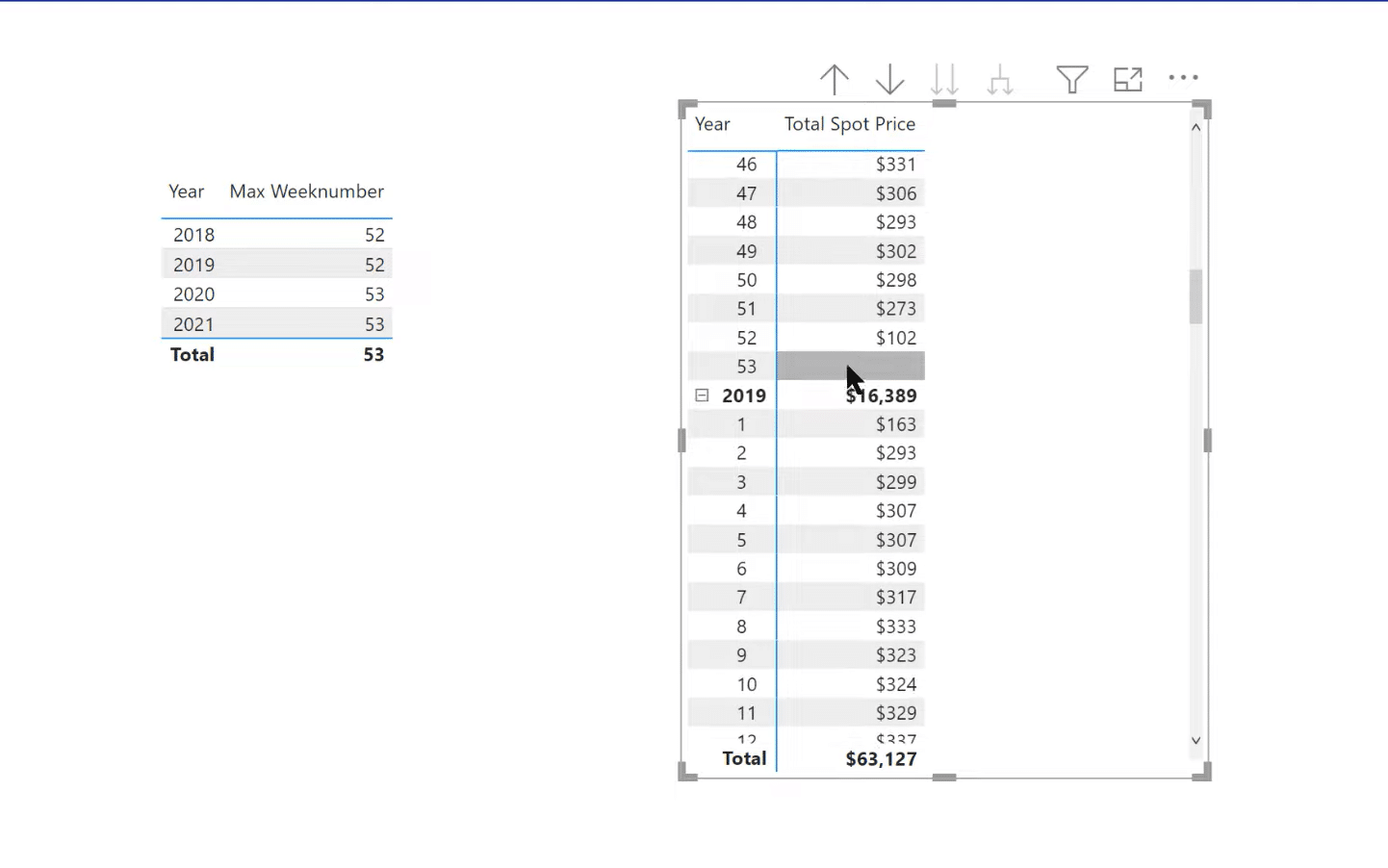
In this case, for each of the years, we want to show a line for week 53, whether there was a week 53 in that year or not. So, you can see in 2018 and 2019, there is no week 53, but in 2020, there is. We want to have it consistent so that the 53rd line would be in each year. But then, the metric would be blank for the years in which there wasn’t a 53rd year.
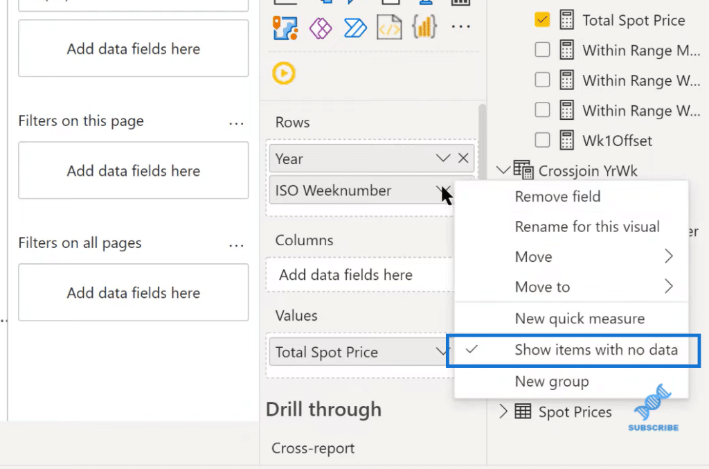
One of the common ways we do that is to go Show items with no data and make sure it’s turned on. In this case, it’s turned on, but it’s not going to help because that works when you’ve got a physical row, but just no data associated with that row. In this case, we don’t even have the row.
Techniques like using ALL or Remove Filters aren’t going to work because there’s nothing to remove. The filter on that row just doesn’t exist. And so, the question is how do we insert that row into each year in which it doesn’t exist? And then, this really becomes a data modelling problem.
One of the things we can potentially do is go to a snowflake scheme where we filter the Dates table by something that will force that 53rd week into our visual each year. The function that jumps to mind for this is CROSSJOIN.
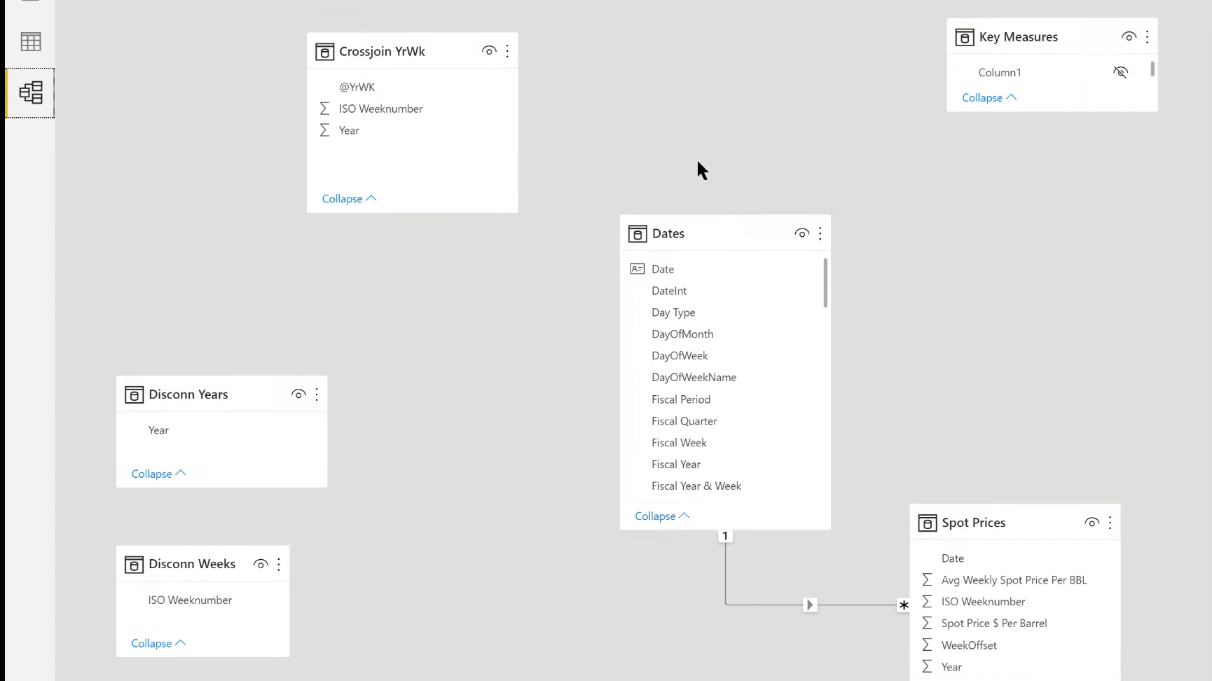
CROSSJOIN is used to match two fields together that may or may not have a relationship. They don’t have to have a relationship unlike most SUMMARIZE or SUMMARIZECOLUMNS, or other table functions.
In this case, CROSSJOIN takes two columns and creates every combination of those two columns, whether that exists in the data set or not. That’s exactly what we want.
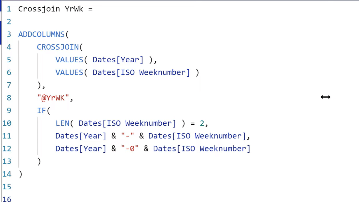
We’ve got our VALUES to create a table out of the column. CROSSJOIN takes two tables and then VALUES on the ISO week number, and we just match those together. That’s going to give us 53 weeks each year.
And then, we’re adding a third column to the table. We could do this in Power Query, but it’s just easier to show you the logic in DAX. What we’re doing here is we’re actually taking and concatenating the Year with a hyphen, and then the week number, so that we’ve got a key field to join it to the Dates table.
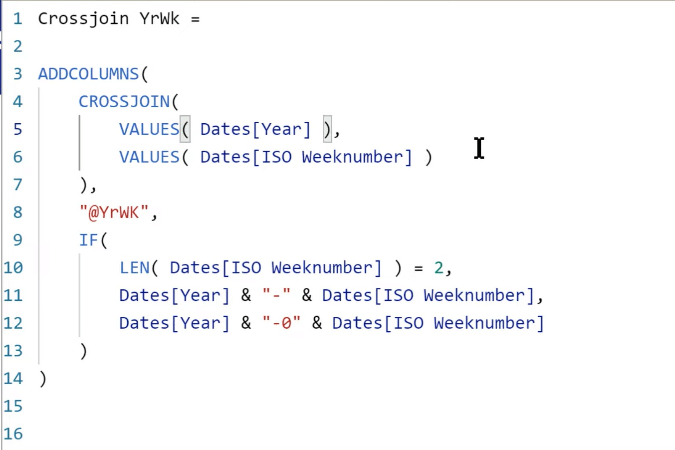
However, we have to do a little more work here because the way that the key field works in the Dates table is it’s a four-digit Year hyphen and then a two-digit week. So, in cases where the ISO week number is two digits, we can just do the simple concatenation. In cases where it’s one digit, we need to take the year number and then concatenate that with a hyphen, then a leading zero, and then the week number.
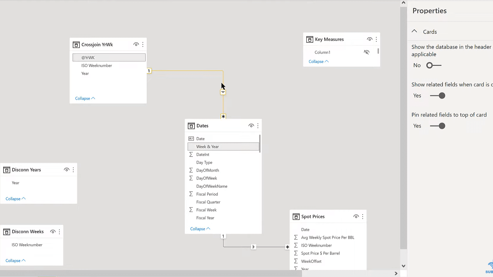
Once we’ve got that, we can take that table in the data model and find our Week & Year column. Then, we join those in a one-to-many relationship. I always like to turn this option on Pin related fields to top of card so that when we check it, we can see it right away.
If we go back to the visual, we’ve got to change the rows. Instead of Year & Week number, we want to use the Year & Week number from the CROSSJOIN table. And now, we’ve got that 53rd week in 2018 with a blank, and the 53rd week in 2019 with a blank. In 2020, we have an actual number since it has the 53rd week.
We could stop here, except for the fact that we’ve now moved out of the Star Schema model. Anytime you move away from the Star Schema in Power BI, you’re moving outside the realm of what’s generally considered best practice.
And so, for Snowflake Schema, it’s not a huge violation. There are cases where you may definitely want to use it, but if you can avoid it, try to. It does reduce duplication, but not necessarily size. It lets you use straight count measures, but there are performance issues and potential usability issues, and definitely increases in DAX complexity. It prevents you from building hierarchies across tables, and probably the most problematic is that it can really mess up your ability to sync slicers across different fields.
So, while this solves the problem, it does so in a way that isn’t great. Let’s see if we can do better than this. Let’s hop into another data model. In this model, I’ve taken the exact same data, the dates and the spot price, but this time I’ve removed the CROSSJOIN table. It does still exist, but it’s not connected.
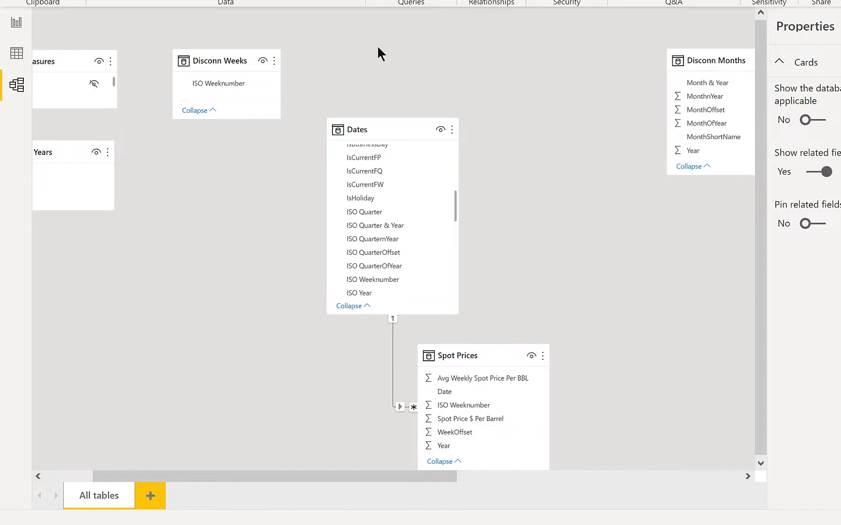
But if we look at the DAX, we’ll see that it’s the exact same DAX that created that table in the other report. So, instead of connecting it in a physical relationship, and then violating the Star Schema, and converting that into a Snowflake Schema, we can maintain the Star Schema and just use a virtual relationship.
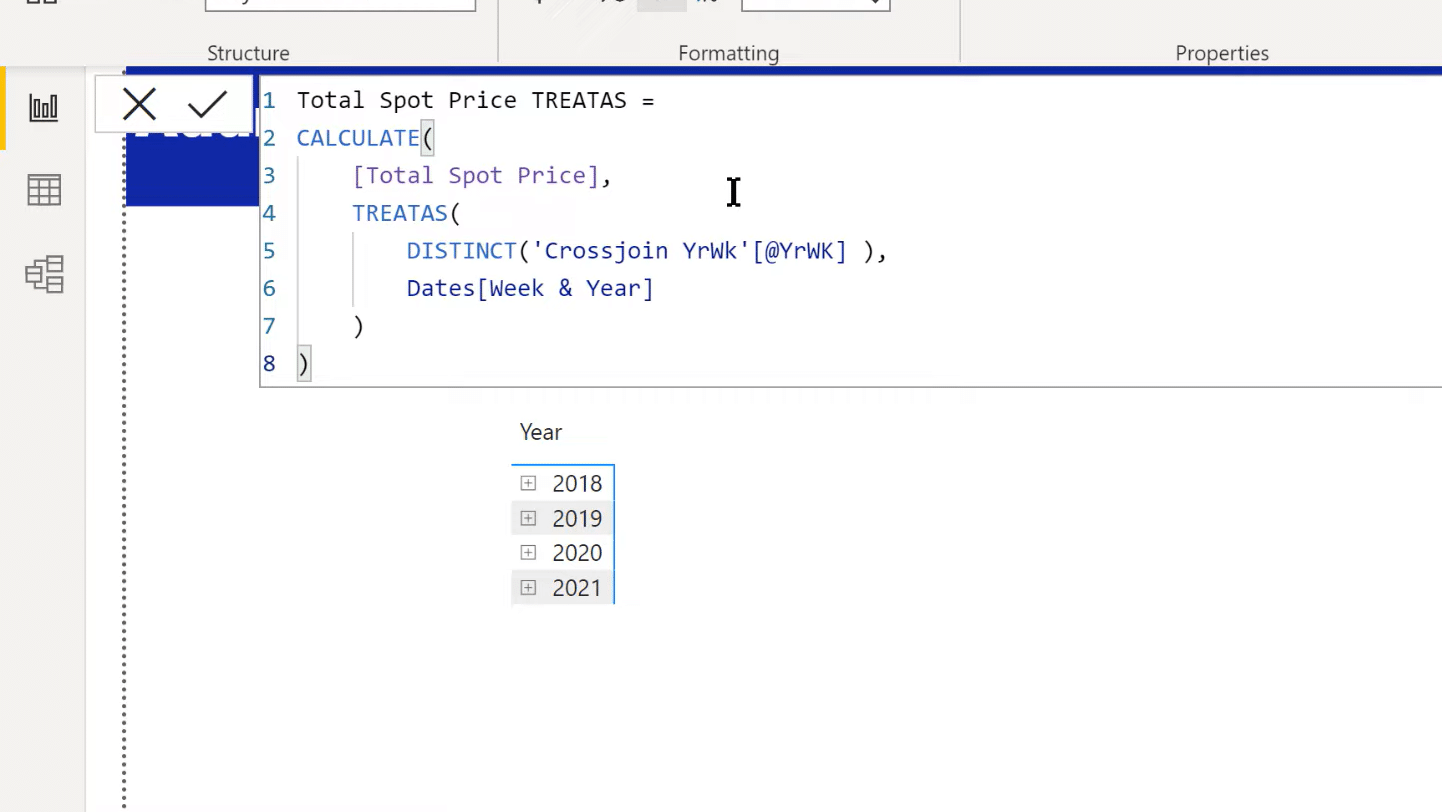
To do that, we’ll use a function called TREATAS. It creates that relationship between tables but does so virtually. We do that using CALCULATE because we’re going to be changing the context. In this case, the context is going to be with regard to the relationship. So, we’ve got our Total Spot Price, and then we’ve got TREATAS. We’ve got the DISTINCT to turn that column into a table.
And then, we’ve got the Year & Week field, which is the key that we created. We’ve got that joined in a virtual way to Week & Year in the Dates table. So now we’ve got that Crossjoint table filtering the Dates table in the same way that it did when we had a physical relationship, but without violating the Star Schema.
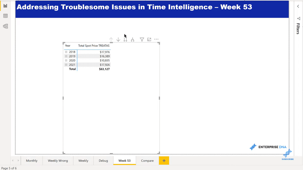
We can now take and drop that Total Spot Price TREATAS into the matrix and what we see is the exact same totals. In this way, we’ve done so without disrupting our data model and incurring any of the disadvantages that we talked about in relation to the Snowflake Schema.
***** Related Links *****
Get Power BI Previous Week Values Using DAX & Power Query
Calculating Weekly Sales w/DAX In Power BI
Time Intelligence In DAX: How To Dynamically Select Starting Period
Conclusion
In this tutorial, I’ve shown you a couple of ways to address the DAX weekly calculation issue in Power BI. One is by using CROSSJOIN, but it has some disadvantages. The second way is by using TREATAS, creating a virtual relationship, and not violating the Star Schema approach.
That is one technique that is quite useful for dealing with that week 53 problem. I hope you found that useful. I want to know your thoughts on this. Let me know in the comments below.
All the best,
Brian


