Big O Calculator: Top Solution for Big O Notation Creation

When writing efficient code, the Big O notation is a programming concept that can help you measure your algorithms’ time and space complexity.

A big O calculator is a time-saving, efficiency-enhancing tool for estimating the time required for tricky sorting instructions. It basically uses Python to help you find algorithm complexity.

This blog post will show you how to use a simple Big O calculator in Python to test how your algorithms scale with different input sizes.

It’s quick, easy, accurate, and effective.

So stick around as we introduce you to Big O notation, automated!

Let’s get started!

The Significance of Big O Notation

Big O notation is a mathematical representation that describes the upper bound of an algorithm’s time and space complexity concerning its input size.

It allows developers to make informed decisions about algorithm selection, helping ensure that programs run efficiently, even as input data grows.

Let’s take a look at the advantages of understanding this concept.

Top 4 Advantages of Understanding Big O Notation

1. Performance Assessment: Big O notation provides a systematic way to assess the performance of algorithms. It helps you predict how an algorithm will behave as the size of the input data increases.

2. Optimization: By analyzing algorithms’ time and space complexity, you can identify bottlenecks and areas for improvement in your code.

3. Algorithm Selection: When faced with multiple ways to solve a problem, Big O notation aids in selecting the most suitable algorithm.

4. Scalability: Understanding Big O notation is crucial for building scalable applications. It ensures that your software can handle larger datasets and maintain optimal performance.

Next up, Let’s explore the steps to create a Big O calculator in Python.

Building a Big O Calculator in Python

This section will walk through an actual example of building a Big O calculator in Python. We’ll apply the steps outlined earlier to create a tool that calculates the time complexity of a specific algorithm.

Let’s dive into the step-by-step process:

Step 1: Define the Problem

In this step, we’ll define the problem we aim to solve. For our example, we’re addressing a common computational task:

• Problem Statement: Calculate the sum of all numbers in an array.

• Input: An array of integers (e.g., [1, 2, 3, 4, 5]).

• Expected Output: The sum of all elements in the array (e.g., for [1, 2, 3, 4, 5], the output should be 15).

Key Considerations:

• What is the most efficient way to sum an array of integers?

• How does the size of the array affect the algorithm’s performance?

• Is there a need to consider edge cases, such as empty or vast arrays?

Clearly defining the problem establishes a solid foundation for developing an effective algorithm.

Step 2: Implement the Algorithm

We’ll implement a straightforward algorithm to calculate the sum of an array in Python.

def sum_array(arr):
    total = sum(arr)
    return total

Ensure the algorithm works correctly and produces the desired results for different input arrays.

Step 3: Measure Execution Time

To measure the execution time, we’ll use Python’s time module. We’ll create input arrays of varying sizes and record the time it takes to compute the sum.

import time

def measure_execution_time(arr):
    start_time = time.time()
    result = sum_array(arr)
    end_time = time.time()
    execution_time = end_time - start_time
    return execution_time, result

Step 4: Analyze and Log Space Complexity

In this step, we’ll analyze the algorithm’s space complexity and implement a way to log or print the memory usage to provide a clear understanding of the algorithm’s requirements.

For our sum_array function:

def sum_array(arr):
    total = sum(arr)
    return total

• The space complexity is centered around the total variable, a single integer. This suggests that our algorithm has a constant space complexity, O(1).

• To observe the memory usage in action, we can use Python’s sys module to monitor and print the usage of our algorithm.

Here’s how you can implement this:

import sys

def sum_array(arr):
    total = sum(arr)
    # Log the usage
    print(f"Mem usage for summing arr.: {sys.getsizeof(total)} bytes")
    return total

# Example usage
sum_array([1, 2, 3, 4, 5])

In this implementation, sys.getsizeof(total) is used to log the size of the total variable. This allows us to observe the actual consumption of the algorithm in bytes, which remains constant regardless of the array size.

By logging or printing the usage, we gain tangible insights into the space efficiency of our algorithm, making our analysis more concrete and actionable.

Step 5: Create Test Cases

Develop test cases with different input sizes to comprehensively evaluate the algorithm’s performance. For example:

input_array_small = [1, 2, 3, 4, 5]
input_array_large = list(range(1, 10001))

Now, we’ll implement the big O calculator.

Step 6: Implement the Big O Calculator

Create a Python script that calculates and displays the Big O notation for the algorithm based on the measurements you collected.

In this case, since the algorithm’s execution time increases linearly with the input size, the Big O notation would be O(n), where ‘n’ is the size of the input array.

def calculate_big_o(arr):
    execution_time, _ = measure_execution_time(arr)
    return f'O(n) - Execution Time: {execution_time:.6f} seconds'

input_array_small = [1, 2, 3, 4, 5]
input_array_large = list(range(1, 10001))

print(calculate_big_o(input_array_small))
print(calculate_big_o(input_array_large))

By following these steps, you’ve built a simple Big O calculator in Python to assess the time needed to execute a particular task.

Let’s take a look at a visualization.

Visualization of the Big O calculator

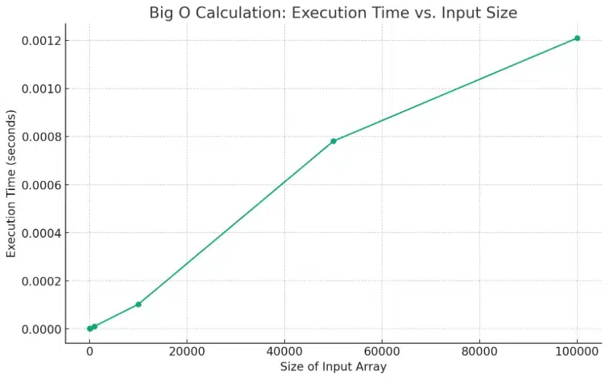
Here’s the visualization of the Big O calculator, showing the relationship between the execution time and the input array size.

As you can see from the graph, the execution time increases as the size of the input array grows. This graphically illustrates the linear relationship, indicative of O(n) complexity, where ‘n’ represents the size of the input array.

You can now use this tool to analyze and optimize your operations, gaining valuable insights into your code’s efficiency.

Feel free to explore more complex implementations and enhance your understanding of Big O notation and algorithmic complexity.

Moving on, let’s take a deeper look at analyzing algorithm performance.

Analyzing Algorithm Performance

Now, let’s explore common time complexities and provide Python code examples to illustrate them:

Constant Time (O(1))

Algorithms with constant time complexity have a fixed execution time, regardless of the input size. This means they perform operations in a constant number of steps. A classic example is accessing an element by index in an array.

def access_element(arr, index): return arr[index]

Logarithmic Time (O(log n))

def binary_search(arr, target):
    left, right = 0, len(arr) - 1
    while left <= right:
        mid = (left + right) // 2
        if arr[mid] == target:
            return mid
        elif arr[mid] < target:
            left = mid + 1
        else:
            right = mid - 1
    return -1

Algorithms with logarithmic time complexity often divide the problem into smaller subproblems and work efficiently on each subproblem. Binary search is a classic example of O(log n) complexity.

Linear Time (O(n))

def linear_search(arr, target):
    for i in range(len(arr)):
        if arr[i] == target:
            return i
    return -1

Algorithms with linear time complexity have a runtime that increases linearly with the input size. An example is a simple linear search.

Quadratic Time (O(n^2))

def bubble_sort(arr):
    n = len(arr)
    for i in range(n):
        for j in range(0, n - i - 1):
            if arr[j] > arr[j + 1]:
                arr[j], arr[j + 1] = arr[j + 1], arr[j]

Algorithms with quadratic time complexity have a runtime that increases with the input size. An example is the bubble sort algorithm.

Comparison Of Algorithm Time Complexities

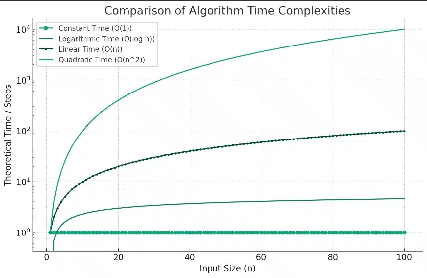
These fundamental time complexities provide a foundation for understanding more complex algorithms and their performance characteristics.

Moving on, let’s take a deeper look at managing memory usage.

Managing Space Complexity

Space complexity(Memory Usage) is equally important in algorithm analysis. Let’s discuss concepts related to space complexity and provide Python code examples:

Auxiliary Space

This represents the extra memory space an algorithm uses beyond the input data. For example, consider the space complexity of a function that computes the factorial of a number.

def factorial(n):
    if n == 0:
        return 1
    else:
        return n * factorial(n - 1)

In this case, the auxiliary space is the memory used to maintain the recursive call stack.

In-Place Algorithms

In-place algorithms minimize memory usage by modifying the input data rather than creating additional data structures. For instance, consider the in-place implementation of reversing an array.

def reverse_array(arr):
    left, right = 0, len(arr) - 1
    while left < right:
        arr[left], arr[right] = arr[right], arr[left]
        left += 1
        right -= 1

This algorithm reverses the array without allocating extra memory for a new array.

Recursive Factorial vs In-Place Array Reversal

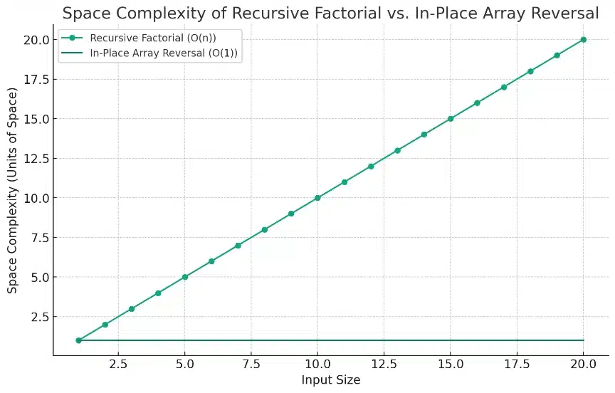
• Recursive Factorial (O(n)): The line representing the recursive factorial function shows a linear increase in space complexity with the input size. This is due to the growing call stack in each recursive call, where the recursion depth equals the input size.

• In-Place Array Reversal (O(1)): The space complexity for the in-place array reversal remains constant regardless of the input size. This is depicted by the flat line, indicating that the algorithm uses a fixed amount of space.

Understanding both time and space complexity and their practical implications is crucial for designing efficient algorithms and making informed decisions in software development.

Finally, let’s reflect on some of the main points.

Final Thoughts

In summary, understanding the Big O notation, analyzing algorithm performance, and grasping expected time and space complexities are essential skills for any software developer.

By considering best-case, average-case, and worst-case scenarios, you can gain a holistic view of an algorithm’s behavior under different conditions.

This knowledge enables you to make informed algorithm selection and optimization decisions, ensuring our programs run efficiently even as input data scales.

In software development, where every millisecond counts, these skills are invaluable. They empower us to build faster, more efficient, scalable software solutions.

So, the next time you face an algorithmic challenge, remember the significance of Big O notation and algorithm analysis – they are your tools for success in coding.

Happy coding!

Want to see how you can use AI for your code? Checkout our latest clip below.

Frequently Asked Questions

What does “big theta” mean in algorithm analysis?

Big Theta (?) notation describes the tight bound of an algorithm’s time complexity. It represents the upper and lower bounds, indicating that the algorithm’s runtime grows at a specific rate.

What is exponential time complexity, and why is it important to avoid it?

This (O(2^n)) occurs when an algorithm’s runtime doubles with each increase in the input size. It’s crucial to avoid because it leads to prolonged performance for more significant inputs. Efficient algorithms aim for polynomial time complexities (e.g., O(n^2), O(n^3)) or better.

How do “for loops” affect algorithm performance?

The number of iterations in a loop directly affects the algorithm’s runtime. Nested loops, for example, can lead to quadratic time complexity (O(n^2)) or worse. Careful loop design is essential for optimizing algorithms.

What is the significance of “big omega” in algorithm analysis?

Big Omega (?) notation represents the lower bound of an algorithm’s efficiency. It indicates the best-case runtime scenario. Understanding big omega helps us identify scenarios where an algorithm performs exceptionally well, even in the most favorable conditions.

Do functions’ parameters and arguments matter in Algorithm Efficiency?

Yes, the number of function parameters and arguments can affect performance. If an algorithm repeatedly calls functions with extensive argument lists, it can impact runtime. Evaluating the impact of function calls on an algorithm’s performance is essential for accurate analysis.

How does the length of input data affect Computational Cost?

Algorithms may have different behaviors depending on input size. Understanding how an algorithm scales with input length is vital for predicting performance.

Is it essential to compare values within an algorithm to determine computational complexity?

Comparing values within an algorithm, especially in loops and conditional statements, is essential for understanding why things run as long as they do. The number of comparisons directly influences the algorithm’s runtime, making it a crucial analysis aspect.

What should I do if I encounter algorithms with high time complexity?

If you encounter algorithms with high time complexity (e.g., exponential or factorial), consider optimizing them. Look for alternative algorithms or strategies, as high complexity can lead to poor performance for significant inputs.

Are there Python libraries or methods that can help optimize algorithms?

Yes, Python offers libraries and built-in functions that implement efficient algorithms and data structures. Leveraging these libraries and functions can often lead to significant performance improvements in your code.

Are there any Python-specific words or concepts to consider in algorithm analysis?

Python-specific concepts may include list comprehensions, generator expressions, and built-in functions. Understanding how these Python-specific features impact algorithm performance is essential for practical analysis.