To collapse are column in Excel is simple, straightforward, and something you will need in your Excel toolkit.
To collapse columns in Excel:
Select the column or columns you want to collapse.
Right-click and choose “Hide” from the context menu.
You can also click the “Hide” button in the “Cells” group on the “Home” tab.
Today we will go over the process of collapsing columns in Excel. In fact, there are 4 great methods that we will break down to help you collapse columns quickly and efficiently.
Time to start learning.
4 Methods to Collapse Columns in Excel
In this section, we will go over the following 4 great methods to collapse columns in Excel.
The 4 methods are:
With Grouping
Using The Context Menu
Using The Ribbon
Using Keyboard Shortcuts

Method 1: How to Collapse Columns With Grouping
Collapsing columns in Excel using the Grouping feature allows you to organize your data by hiding certain details while still keeping them accessible.
Follow the steps below to collapse columns using this feature:
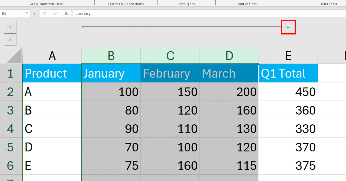
Step 1: Select The Columns
First, select the columns you wish to group.
For instance, if you want to group monthly data columns to focus on quarterly totals, select the columns that represent the months.
Step 2: Group The Columns
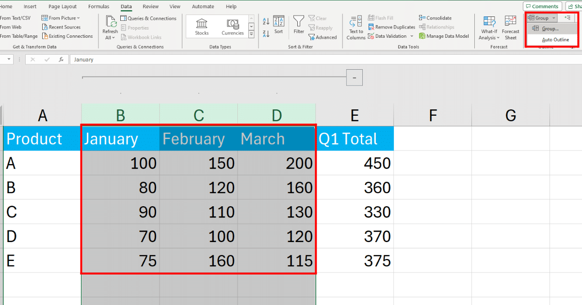
Go to the Data tab on the ribbon, find the Outline group, and click on Group feature.
Then, click “Group” again in the dropdown menu. Excel will add a grouping outline to these columns.
Step 3: Collapse the Group
Once the columns are grouped, you’ll see a box with a minus (-) sign above your selected columns in the outline bar.
Click the minus sign to collapse the group.

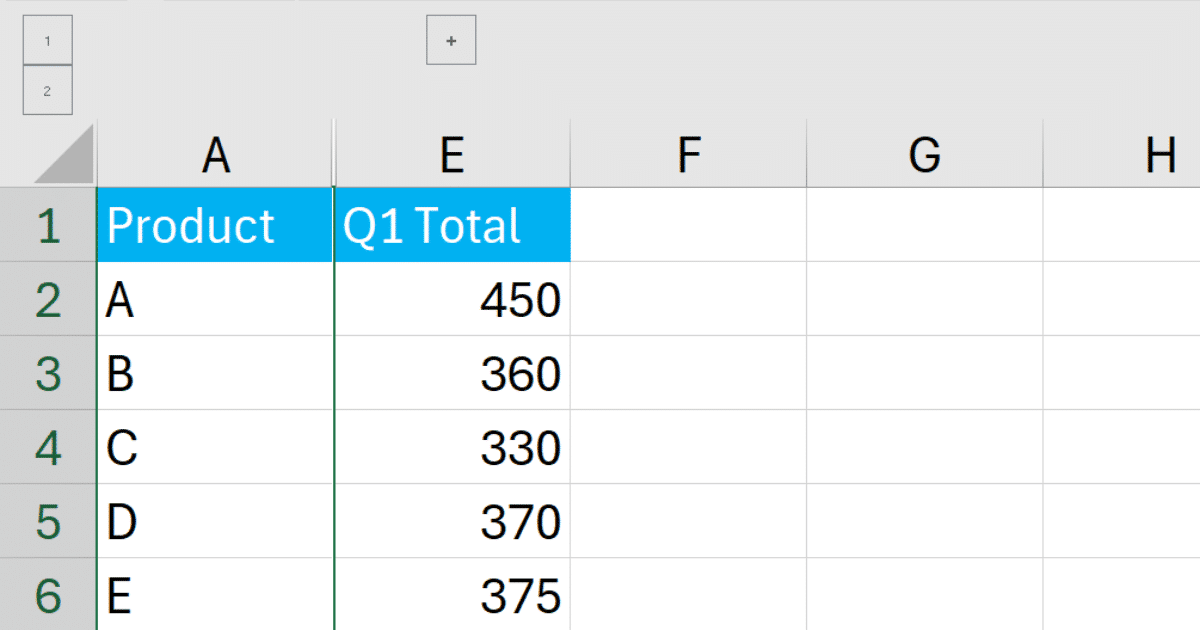
This action will hide the monthly data and only show the Q1 totals.

Method 2: How to Collapse Columns Using The Context Menu
Collapsing columns in Excel by hiding them with the context menu is a straightforward method to simplify your view without altering the structure of your data.
Follow the steps given below to collapse columns using this method:
Step 1: Select Columns to Hide
Select all the columns or data range that you want to hide.
Step 2: Hide the Columns
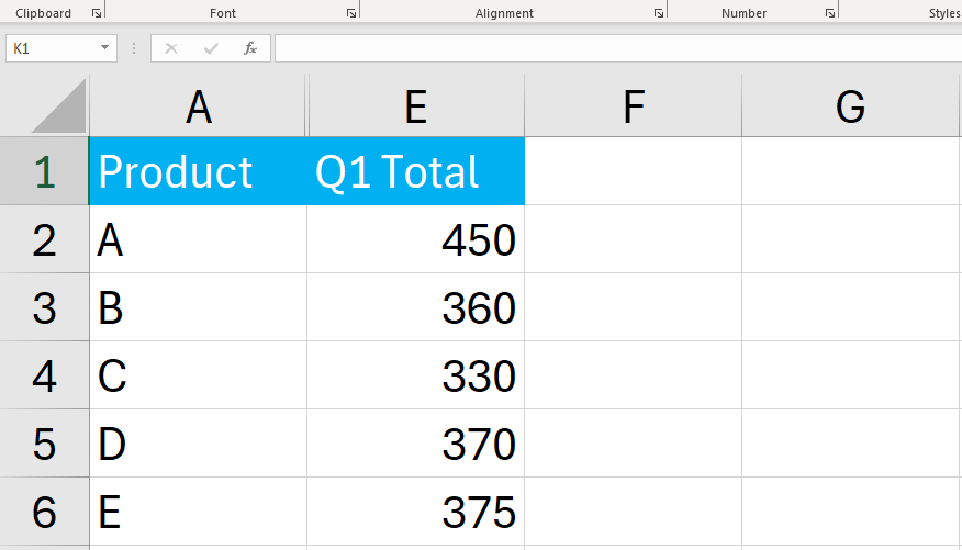
With the columns selected, right-click on one of the selected column headers and choose Hide from the context menu.
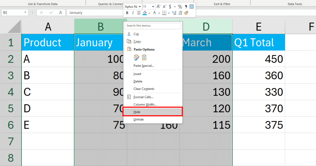
When you click Hide, Excel will hide the selected columns from the view.
Method 3: How to Collapse Columns Using The Ribbon
Another method to collapse columns in Excel is to use the Format feature on the ribbon.
Follow the steps below:
Step 1: Select The Data
Select all the columns that you would like to hide from the view.
Step 2: Hide The Columns
You can go to the Home tab on the Excel ribbon, find the Cells group, click on Format, point to Hide & Unhide, and then select Hide Columns.
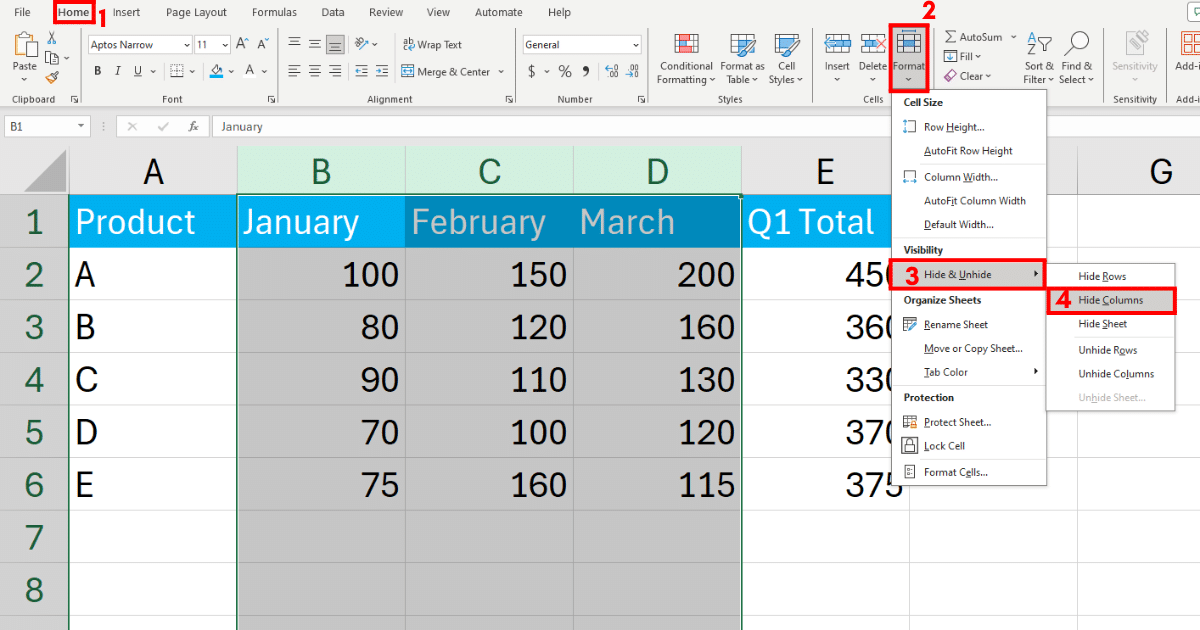
When you click hide, Excel will hide the selected columns from the view.

Method 4: How to Collapse Columns Using Keyboard Shortcuts
Collapsing columns in Excel using keyboard shortcuts streamlines your workflow by reducing the reliance on mouse navigation.
Follow the steps given below to collapse columns using keyboard shortcuts:
Step 1: Select Columns
Select all the columns that you wish to hide.
Step 2: Hide Columns
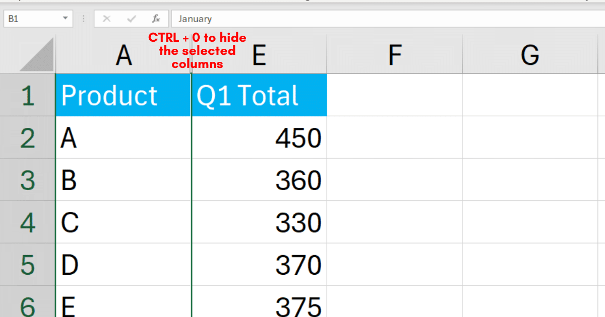
Once the columns are selected, press Ctrl + 0 (zero) to hide them. This shortcut instantly hides the selected columns without needing to access the context menu or the ribbon.
Learn how to count distinct values in Excel by watching the following video:
Final Thoughts
Whether you’re dealing with complex spreadsheets or simply want to focus on specific areas, the ability to hide or group columns comes in handy.
By mastering the techniques you’ve learned today, you can create cleaner, more organized workbooks that are easier to read and work with.
So, next time you’re working on an Excel project, remember the power of collapsing columns and use it to your advantage!
Frequently Asked Questions
In this section, you will find some frequently asked questions you may have when collapsing columns in Excel.

How do I Hide a Column in Excel?
To hide an entire column in Excel, simply select the column or columns you want to hide, right-click, and choose “Hide” from the context menu.
You can also go to the “Home” tab, click “Format” in the “Cells” group, and select Hide & Unhide followed by “Hide Columns.”
What is the Shortcut to Hide Columns in Excel?
The shortcut to hide columns in Excel is “Ctrl + 0” (zero). To use this shortcut, select the column or columns you want to hide, and then press “Ctrl + 0.” If you’re using a Mac, the shortcut is “Cmd + 0.”
How do I Unhide a Column in Excel?
To unhide a column or multiple columns in Excel, first, select the adjacent columns to the hidden column. For example, if you want to unhide column C, select columns B and D. Then, right-click on one of the selected column letters and choose “Unhide” from the context menu.
What is the Shortcut to Unhide Columns in Excel?
The shortcut to unhide columns in Excel is “Ctrl + Shift + 0” (zero). To use this shortcut, first, select the adjacent columns to the hidden column, including the columns on both sides of the hidden column. Then, press “Ctrl + Shift + 0.” On a Mac, the shortcut is “Cmd + Shift + 0.”
How do I Group Rows in Excel?
To group rows in Excel, first select the rows you wish to group. Then, navigate to the Data tab on the Excel ribbon, and in the Outline section, click on “Group.” This step is crucial for grouping rows.
This will group your selected rows, making them collapsible and expandable with a click.
How to Collapse Multiple Columns in Excel?
To collapse multiple columns in Excel, first group them by selecting the columns, then go to the Data tab and click Group in the Outline section.
Once grouped, click the minus (-) sign on the grouping bar above the columns to collapse them.


