An Excel if function with three conditions engages the program to perform a logical test against multiple criteria and return different results based on the satisfaction of said conditions.
To use an IF function with three conditions in Excel, you can nest IF statements inside each other. Start with the first condition, and for the false part of each IF, nest the next IF statement.
This function plays a critical role in streamlining data analysis by enabling users to perform comprehensive evaluations with varied outcomes expressed as literals, references, numbers, or even further functions.
This article will show you how to use an IF function with 3 conditions in Excel. We will break the process down into multiple steps with demonstrations to help you better understand the concepts.
Let’s get started!

What is AN IF Function
The IF function in Excel is a logical function used to perform conditional tests on values and formulas.
It evaluates a given condition to return one value if the condition is TRUE and another value if the condition is FALSE.
The basic syntax of the IF function is:
=IF(logical_test, value_if_true, value_if_false)logical_test is the condition you want to check.
value_if_true is the value that is returned if the condition is true.
value_if_false is the value that is returned if the condition is false.
4 Methods to Use IF Function With 3 Conditions
In this section, we will go over 4 methods of using IF function with 3 conditions.
The methods are:
Nested IF Function
IF With AND/OR
IFS Function
IF With Match

1. How to Use Nested IF With 3 Conditions
To use nested IF functions with three conditions in Excel, you’ll create a formula where each IF statement is placed inside the false value argument of the previous IF.
This allows you to evaluate up to three conditions sequentially.
The basic structure is:
=IF(condition1, value_if_true1, IF(condition2, value_if_true2, IF(condition3, value_if_true3, value_if_false3)))Example
Suppose we have the following dataset:
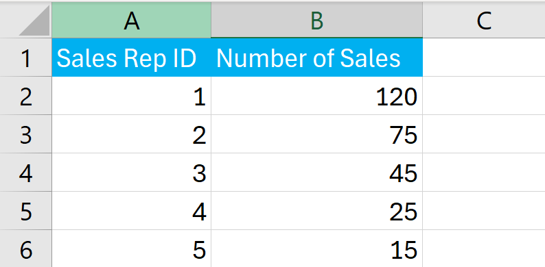
Assume you’re evaluating the performance of sales reps based on the number of sales they make such that:
High if sales are greater than 100.
Medium if sales are between 51 and 100.
Low if sales are between 21 and 50.
Needs Improvement if sales are 20 or less.
Given the number of sales in cell B2, the following formula categorizes the performance of the sales rep:
=IF(B2 > 100, "High", IF(B2 > 50, "Medium", IF(B2 > 20, "Low", "Needs Improvement")))This formula checks the number of sales against each condition in turn and categorizes the sales rep accordingly.
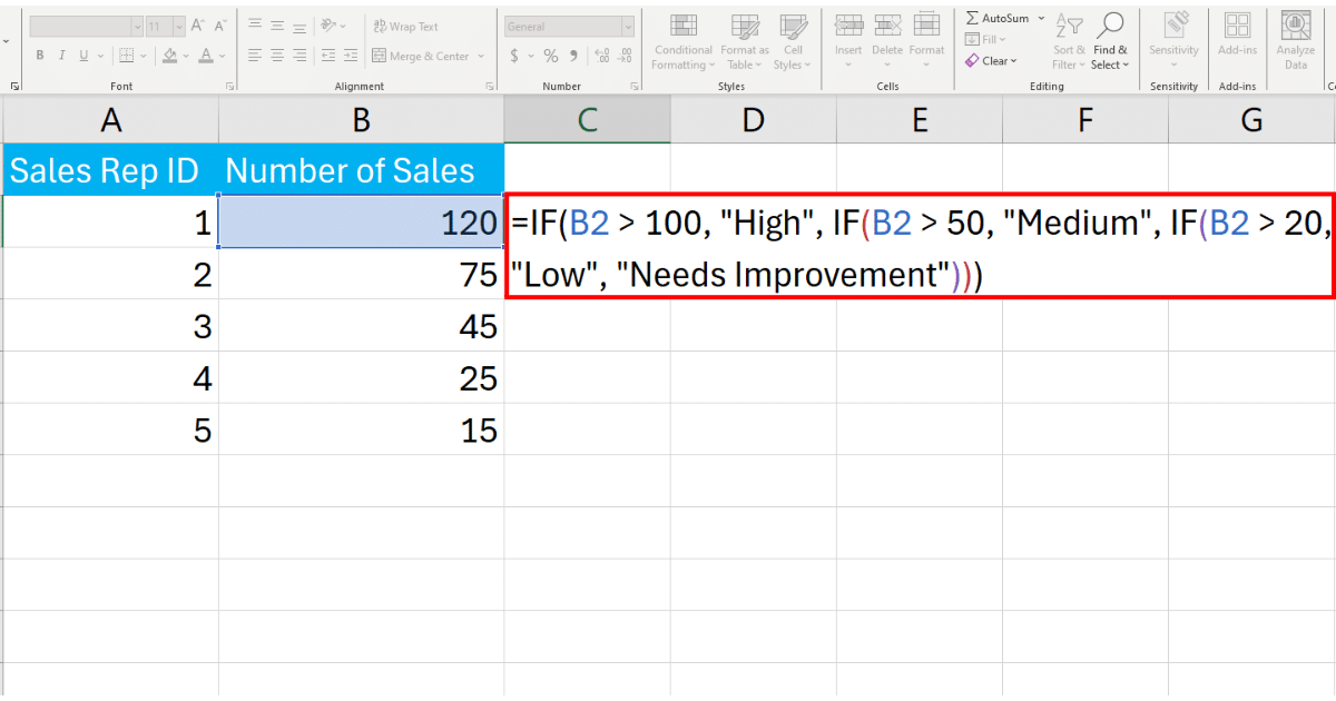
Press Enter and Excel will categorize the sales rep. Drag the fill handle down to apply the formula to the rest of the column as well.
2. How to Use IF With AND/OR For 3 Conditions
To use the IF function with the AND/OR function for evaluating three conditions in Excel, you can combine these logical functions within an IF statement to test multiple conditions at once.
AND requires all conditions to be true for the result to be true, while OR requires any one of the conditions to be true for the result to be true.
Using IF With AND
The general structure of using IF with AND is as follows:
=IF(AND(condition1, condition2, condition3), value_if_true, value_if_false)Suppose you want to determine whether a sales representative achieves multiple objectives, such as sales above 100 units, customer satisfaction above 80%, and a product knowledge score over 90.
The dataset is given below:
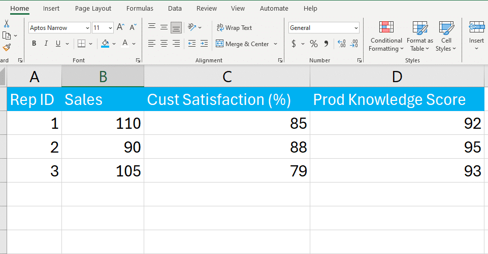
The formula for this scenario will be:
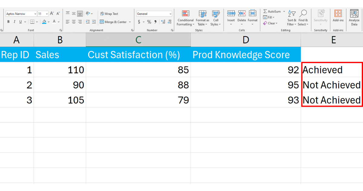
=IF(AND(B2 > 100, C2 > 80, D2 > 90), "Achieved", "Not Achieved")In Excel, the formula looks like the following:
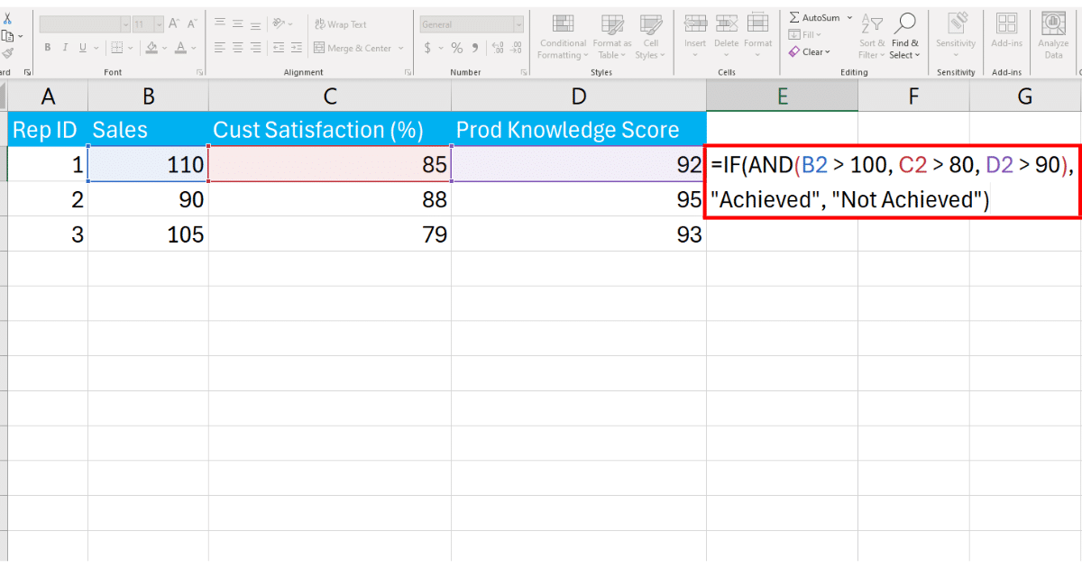
Press Enter and Excel will display the result. Drag the fill handle down to apply the formula to the rest of the column as well.

This approach ensures that only those meeting all benchmarks are recognized as having “Achieved” their goals.
Using IF With OR
The general syntax for using IF with OR is:
=IF(OR(condition1, condition2, condition3), value_if_true, value_if_false)Suppose we have a scenario where a student needs to pass at least one of three subjects to advance, with passing defined as a score above 60.
The dataset is given below:
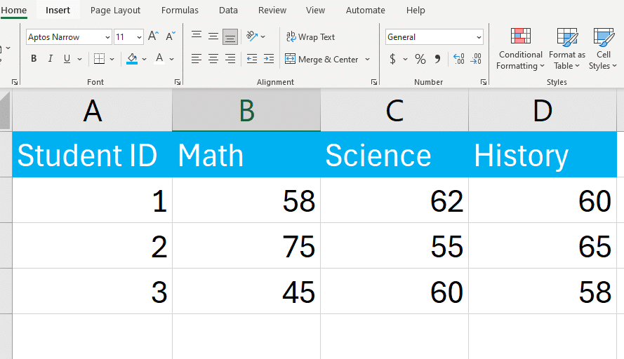
The formula for this scenario will be:
=IF(OR(B2 > 60, C2 > 60, D2 > 60), "Advance", "Retake")In Excel, the formula looks like the following:

Press Enter and Excel will display the result. Drag the fill handle down to apply the formula to the rest of the column as well.

This scenario acknowledges the varied strengths of students, allowing them to move forward based on success in any one area.
3. How to Use IFS Function With 3 Conditions
The IFS function streamlines the process of evaluating multiple conditions without the need to nest IF statements.
It allows you to specify a series of conditions and returns the first true condition’s corresponding value.
The general syntax of IFS is given below:
=IFS(condition1, value_if_true1, condition2, value_if_true2, condition3, value_if_true3)This function tests each condition in order; when a condition evaluates to true, Excel returns the corresponding value for that condition and stops evaluating the rest.
Suppose you want to categorize students based on their scores:
Excellent for scores 90 and above,
Good for scores between 70 and 89,
Average for scores between 50 and 69,
Needs Improvement for scores below 50.
The dataset is given below:

The formula for this scenario will be:
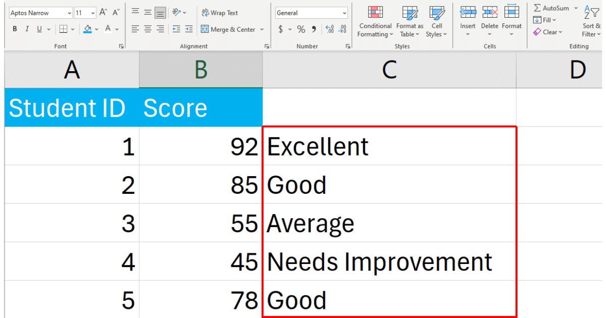
=IFS(B2 >= 90, "Excellent", B2 >= 70, "Good", B2 >= 50, "Average", B2 < 50, "Needs Improvement")In this formula, Excel checks the student’s score against each condition sequentially. It assigns a category based on the first true condition.
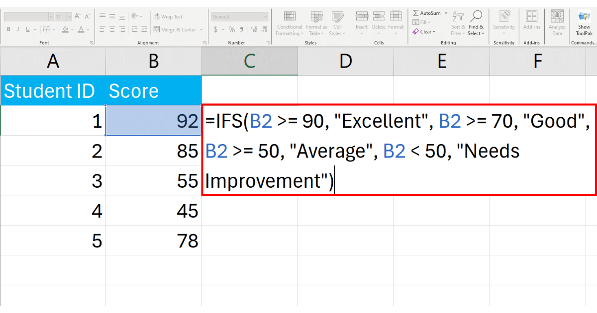
Press Enter and Excel will display the result. Drag the fill handle down to apply the formula to the rest of the column as well.
4. How to Use IF With MATCH For 3 Conditions
The MATCH function searches for a specified item in a range of cells and then returns the relative position of that item.
When combined with IF, you can perform actions based on whether a match is found.
Let’s say you have a list of project codes, and you need to verify if a particular project code matches any of three specific codes to categorize it as “Approved”, “Pending”, or “Rejected”.
The dataset for this scenario is given below:
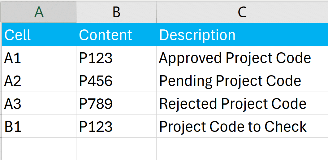
The breakdown of codes is given below:
Code1 (Approved): “P123”
Code2 (Pending): “P456”
Code3 (Rejected): “P789”
You want to check if a project code in cell B2 matches any of the three specific codes and return a status accordingly.
The formula with Excel functions will be:
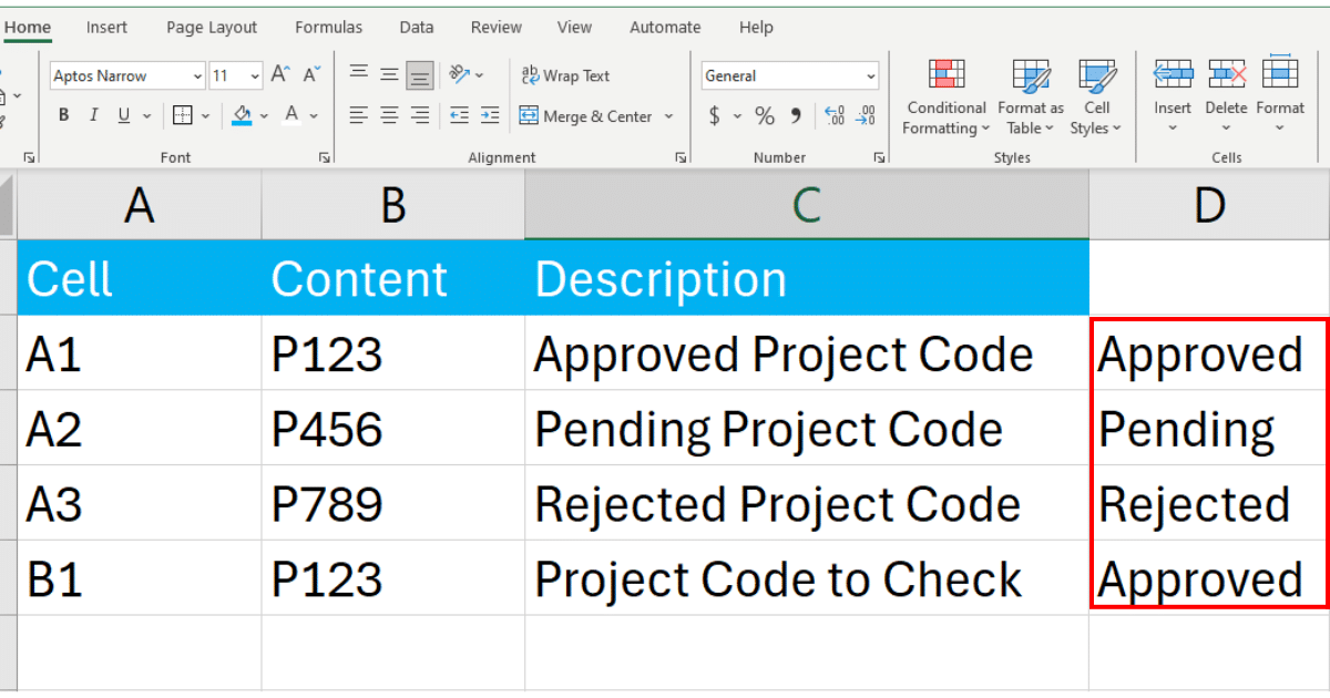
=IF(ISNUMBER(MATCH(B2, {"P123"}, 0)), "Approved", IF(ISNUMBER(MATCH(B2, {"P456"}, 0)), "Pending", IF(ISNUMBER(MATCH(B2, {"P789"}, 0)), "Rejected", "Code Not Recognized")))The formula uses MATCH to search for B2 in each array of specific codes.
ISNUMBER checks if MATCH returns a numeric position (indicating a match was found).
Nested IF statements allow for checking logical tests to return “Approved”, “Pending”, “Rejected”, or “Code Not Recognized” if none of the conditions are met.

Press Enter and function checks will display the result. Drag the fill handle down to apply the formula to the rest of the column as well.
Excel is great, but try and learn how to use ChatGPT for Data Analysis it’s a gamechanger!
Final Thoughts
Employed to its full potential, the power of the nested IF statement can simplify complex decision-making processes, allowing for more efficient data analysis and a clearer visualization of data relationships.
As you gain proficiency in crafting nested IF statements and explore its various uses, you’ll realize the true potential of data analysis and the insights that it can provide.
As you continue to uncover the multitude of applications for the nested IF statement, always remember to structure your logic in a way that is easy to follow and maintain. This approach will enable you to leverage the nesting capabilities of the IF statement and perform even more complex evaluations.
Frequently Asked Questions
In this section, you will find some frequently asked questions you may have when using an IF function with 3 conditions in Excel.

What is an IF formula in Excel?
An IF formula in Excel is a logical function that allows you to perform a test on data and return different results based on whether a specified condition is met.
It is a versatile tool for creating conditional statements in spreadsheets.
How do I write a formula in Excel with multiple conditions?
To write a formula in Excel with multiple conditions, you can use nested IF functions.
Nesting allows you to evaluate several conditions and specify different results for each condition within a single formula.
Can you provide an example of a formula in Excel with multiple conditions?
Certainly! Here’s an example of a formula with multiple conditions:
=IF(A1>90, "A", IF(A1>80, "B", IF(A1>70, "C", "D")))This function Excel checks the value in cell A1 and assigns a letter grade based on the score.
What is the significance of the “position column” in Excel when using IF functions with multiple conditions?
The “position column” refers to the column in your Microsoft Excel spreadsheet where you want to apply the IF formula with multiple conditions.
It specifies where the results of the formula will be displayed based on the conditions you set.
How can I use the AND function to check multiple conditions in an Excel IF formula?
You can use the AND function in conjunction with IF to check multiple conditions simultaneously. The AND function ensures that all specified conditions must be true for the formula to return a specific result.


