We’ll continue our series on Power BI project planning and implementation. This time around, we’ll be discussing on dataset design, profiling, and modes. Check out the first part of our project planning series that deals with deployment modes, and the second part which talks about discovery and ingestion.
Dataset Design For Power BI Project Implementation
Let’s talk about the dataset design process and discuss the data warehouse bus matrix, which is a tool that has been around for a while.
Designing power BI datasets is similar to designing data warehouses. So both datasets and data warehouses have similar concepts such as fact and dimension tables, star schemas, slowly changing dimensions, fact table granularity, and local informed keys for building relationships between tables.
4 Steps to Dataset Design
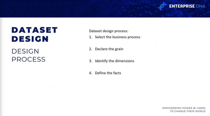
There are four steps to the dataset design process: select the business process, declare the grain of your fact tables, identify the dimensions, and then define the facts.
Select the business process.
For the first step, each business process is represented by a fact table with a star schema of many to one relationship to the dimensions.
During a discovery or requirements gathering process, it is difficult to focus on a single business process in isolation, as users regularly analyze multiple business processes simultaneously.
The Anti-Pattern To Avoid In Power BI Implementation
The common anti-pattern (which is a response to a reoccurring problem that is generally ineffective and potentially counterproductive) that you want to avoid in Power BI projects is the development of datasets for specific projects or teams rather than for the business processes.
For example, developing a dataset exclusively for the marketing team and another dataset for the sales organization. This approach naturally leads to wasted resources because the same sales data is queried and refreshed twice in both data sets. These will also consume storage resources in the Power BI service.
these are some of the reasons why you want to go through a good process for dataset design. An isolated approach leads to manageability and version control issues because the data sets may contain variations and transformations.
Although the analytical needs of the users or teams are the priority of Power BI projects, it’s also important to plan for sustainable solutions that can ultimately be shared across teams.
Declare the grain.
The grain of fact tables ultimately covers the level of detail available for analytical queries, as well as the amount of data that can be accessed.
So higher grain means more detail while lower grain means less detail. An example of this is when you want to get the sales order line level, or if you want the project to only contain the summary level of each sales order and not get down to the specific products that were ordered as part of that sale.
Sometimes, this grain can vary depending upon your timeframe. I’ve come across a number of customers that want very fine-grained fact tables for the current quarter, but for previous quarters, they just needed to know what the total sales for the quarter was.
During this step, you want to determine what each row of the different business processes represent. For example, each row of the sales fact table from our data warehouse represents the line of a sales order from a customer.
Conversely, the rows of a sales and margin plan will be aggregated in a calendar month, product sub-category, and sales territory region. so in this case, you have two different fact tables and two different grains. if you want to compare the two, there will be some data modeling work involved.
Identify the dimensions.
Dimensions are just the natural byproduct of the grain chosen in the previous design step.
So a single sample row from the fact table should clearly indicate the business entity’s dimensions associated with the given process, such as the customer who purchased an individual project, the product on a certain date and at a certain time. Fact tables representing lower grains have fewer dimensions.
For example, a fact table representing the header level of a purchase order may identify the vendor, but not the individual product purchase from the vendor. so in that case, you wouldn’t need a product category or a product subcategory dimension included.
Define the facts.
The facts represent the numeric columns included in the fact tables. So while the dimension columns from step 3 are used for relationships, the fact columns are used in measures containing aggregation logic, such as the sum of a quantity column or the average of a price column.
Data Bus Matrix For Power BI Project Implementation
The data warehouse bus matrix is a staple of the Ralph Kimball data warehouse architecture, which provides an incremental and integrated approach to data warehouse design.
The architecture that you see here is from The Data Warehouse Toolkit, 3rd edition by Ralph Kimball. It allows for scalable data models that multiple business teams or functions often require to access the same business processes and dimensions.
Keeping a data warehouse bus matrix around is useful. when you fill it out, you’ll know if there are other datasets that contain similar internet fact tables and dimension tables. this promotes the reusability of the project and improve project communication.
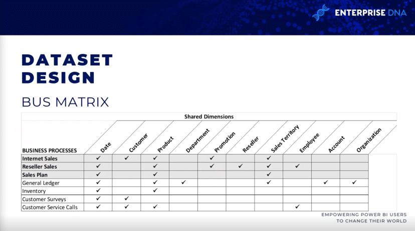
So each row reflects an important and reoccurring business process such as the monthly close of the general ledger. each column represents a business entity, which may relate to one or several of the business processes, while the shaded rows represent the business process that are being included within the project.
Data Profiling For Power BI Implementation
once you’ve identified the grain and the four-step dataset design process has been completed, it should be immediately followed by a technical analysis of the source data of the fact and dimension tables.
Technical metadata, including database diagrams and data profiling results, are essential for the project planning stage.
This information is used to ensure the power BI dataset reflects the intended business definitions and is built on a sound and trusted source.
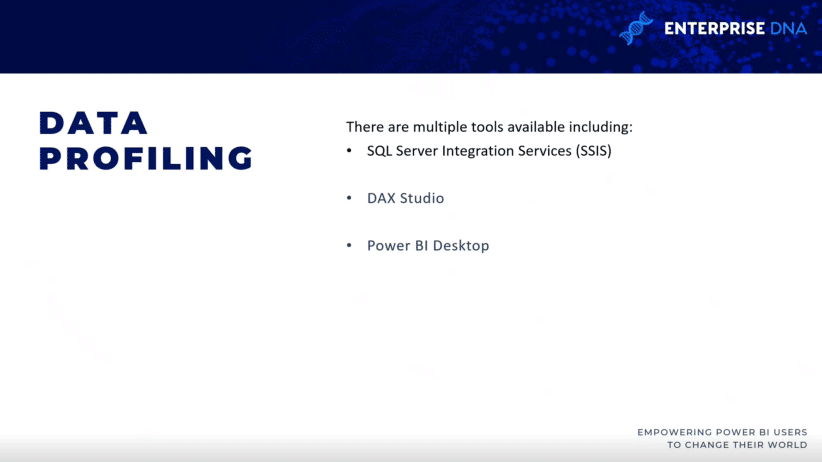
So three are three different ways of collecting that profiling information, which should be the very first step that people will do once they come out of the the design process.
SQL Server Integration Services
There are a couple of ways to go about this. One method is to use a data profiling task within an SQL Server Integration Services (SSIS) package.
The data profiling task requires an a ADO.NET connections and can write its output to an XML file or an SSIS variable.
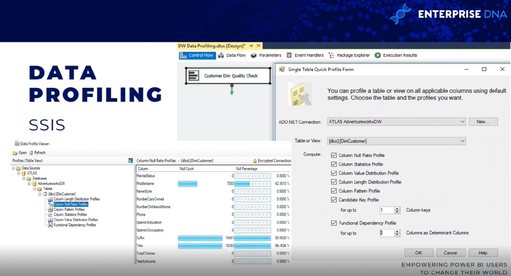
In this example, the ADO.NET source data is an AdventureWorks data warehouse, database, and SQL server, and the destination is an XML file.
So once the task is executed, the XML file can be read via a SQL server data profile viewer. You can see the results in terms of null count and null count percentages.
DAX Studio
Another way of data profiling is via DAX Studio. you have to actually ingest the data into a Power BI dataset by going to DAX Studio, go to the advanced tab, and run the VertiPaq Analyzer.
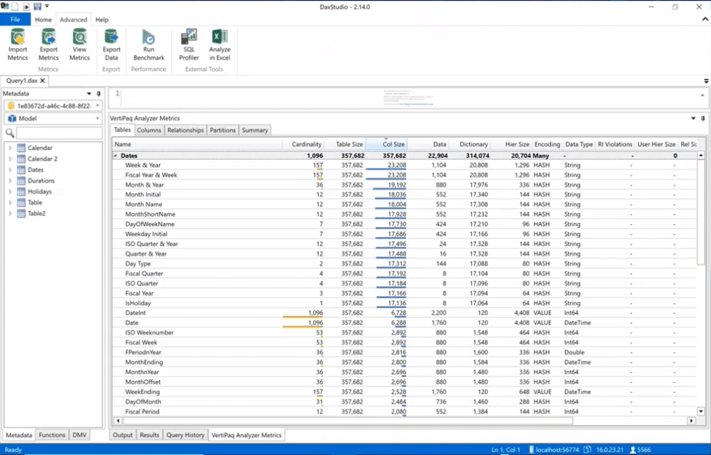
It will show you the same kind of information around the cardinality of your columns so you’ll know which ones are taking up the most space in your data model. it includes all the various statistics around the data.
Power BI Desktop
data profiling is also available in power query within Power BI desktop. if you go to the View tab, you can turn on things like column quality, column distribution, and column profile. For at least the first thousand rows or so, you can see the information such as errors, nulls, averages, and standard deviations.
Dataset Planning For Power BI Implementation
After the source data is profiled and evaluated against the requirements identified in the four-step dataset design process, the BI team can further analyze the implementation options for the dataset.
In almost all power BI projects, even those with significant investments in enterprise data, warehouse, architecture and ETL tools and processes, some level of additional logic, integration or transformation is needed to enhance the quality and value of the source data.
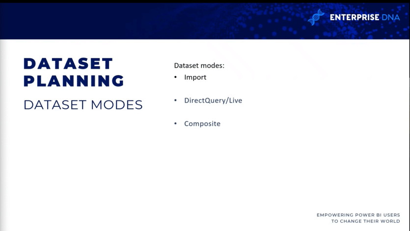
The dataset planning stage determines how the identified data transformation issues are addressed to support the dataset. Additionally, the project team must determine whether to develop an import mode dataset, a direct query dataset, or a composite dataset.
To clarify the dataset planning process, this diagram identifies the different layers of the data warehouse and Power BI dataset where transformation and business logic can be implemented.
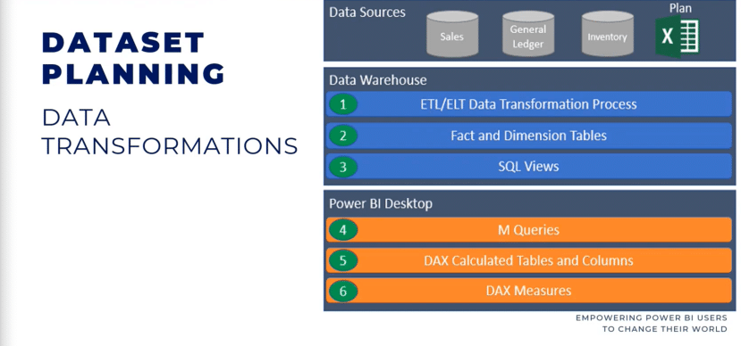
in some projects, minimal transformation is needed and it can easily be included in the power BI dataset. For example, if only a few additional columns are needed for a dimension table and there’s straightforward guidance on how these columns will be computed, the IT organization may choose to implement these transformations within M power queries rather than revise the data warehouse.
If the substantial gap between the BI needs and the corporate data warehouse is allowed to persist, then the Power BI datasets become more complex to build and maintain.
Dataset designers should regularly analyze and communicate the implications of datasets if there is greater levels of complexity.
However, if the required transformation logic is complex or extensive with multiple joint operations, row filters, and data type changes, then the IT organization may choose to implement essential changes in the data warehouse to support the new dataset and future BI projects.
For example, a staging table and a SQL store procedure may be needed to support, revise, and update process, or the creation of an index may be needed to improve query performance for DirectQuery datasets.
Choosing A Dataset Mode
A subsequent but closely related step to dataset planning is choosing between the default import mode, DirectQuery/live mode, or composite mode.
In some projects, this is a simple decision where only one option is feasible or realistic given the known requirements, while other projects will entail significant analysis of the pros and cons of each design.
So if a data source is considered slow or ill equipped to handle a high volume of analytical queries, then an import mode dataset is very likely the preferred option.
Likewise, if near real-time visibility of a data source is essential, then DirectQuery or live mode is the only option to achieve that. the DirectQuery and live modes are very similar to one another. Both methods don’t store data within the dataset itself, and both query the source systems directly to retrieve data based on user action. We now have DirectQuery for Power BI datasets and DirectQuery for Analysis Services.
Some Questions To Ask When Choosing Dataset Modes
Here are some questions to ask when deciding which mode to use. is there a single source for our dataset? If there isn’t a single source, then you couldn’t use DirectQuery/Live source in the past.
Even though we now have composite mode datasets, it’s still a good question to ask at the outset because if there is no single source, then it will either be import or composite.
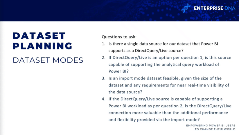
If DirectQuery/Live source is an option, is the source capable of supporting analytical queries? If you’re working with billions or trillions of rows, then maybe an import mode dataset is not feasible and you’ll have to go down the DirectQuery or composite mode to make sure that the dataset is usable.
If the DirectQuery/Live source is capable of supporting the workload, is the DirectQuery/Live connection more valuable than the performance and flexibility provided by an import model?
Conclusion
This post wraps up this series on planning Power BI projects. these, I think, are the essential steps for every power BI projects that you work on. These steps are important when doing the due diligence, especially in an enterprise business intelligence setting.
All the best,
Greg Deckler


