Analyzing the data that we have can be difficult if it is not correctly arranged. In this tutorial, I will explain how to transform vertical and horizontal repeated data into a tabular format. We do this so that we can have an easier time analyzing it using Power BI. You may watch the full video of this tutorial at the bottom of this blog.
This tutorial was made to address the question of an Enterprise DNA Support Forum member. The member asked for a way in which he could remodel his data from a calendar type layout into a tabular format.
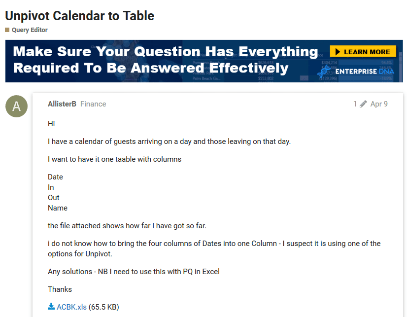
Before we start, let’s first examine the data we have.

Here, we have a data layout wherein the days are set up horizontally, and the weeks are set up vertically. This type of arrangement is familiar to most of us since this is the way we can easily understand the data.
However, this type of layout is harder to analyze since there are many columns and rows to take into consideration.
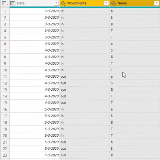
With that being said, let’s transform the data into a proper table format where we end up with a column for dates, a column for the movements, and another column for the names.
Cleaning Up Data For A Proper Tabular Format
To make things easier, let’s transform our data inside the Power Query Editor. But before we do that, let’s make sure that the Formula Bar is visible on your screen. If it’s not, go to the View tab then check the box beside the Formula Bar.

The first step is to remove the unnecessary values in our data. Let’s remove the first column and the top two rows of our data since we don’t really need them. To do that, click on the Remove Rows tab, click Remove Top Rows, enter 2, then press OK.

And now to remove the first column, go to the Choose Columns tab, and then deselect column 1 by unchecking the box next to it.

Let’s also remove rows index 14 to 16 since they are completely filled with just null values. Again, go to Remove Rows tab then click Remove Blank Rows.

Another issue that we have is that the date values skip a column every time. The dates are always followed by a null value as highlighted below. This happens not just on the top row but on the rows below as well.

To fill these gaps, let’s first transpose our data table by going to the Transform tab then clicking the Transpose button.

The table should now look like it has been flipped on its side after performing the action.

Next, select all the columns that contain the dates, right-click the column header, then select Fill Down.

This should duplicate the dates and fill the gaps in the selected columns.
Breaking The Tables
Looking at the data that we now have, we see that there are four tables adjacent to each other. Columns 1 to 7 form one table, columns 8 to 13 form another table, and so on.
To append these into one single table, we need to perform a basic unpivot operation to transform it into a proper tabular format. But since the tables are adjacent to one another, we can’t simply do that. We have to break this table apart and stitch them back together into smaller tables.
To do that, we’ll create the first formula for this tutorial. Let’s click the fx button then add the formula that we’re going to use. We’re going to use the Table.ToColumns operation. This creates a list of nested lists of column values from a table. Each column will be turned into a list.
This is how I’ve set up the formula.

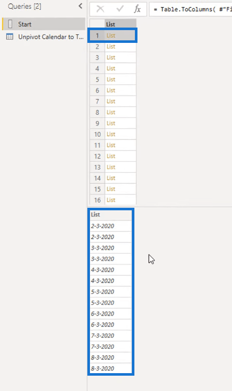
The formula creates a list of the columns that we previously have. The first value of the list contains column 1, the second value contains column 2, and so on.
Identifying The List For The New Tables For A Proper Tabular Format
Now, we should identify which values on the list contain date values. Once we know where these dates are located, we can determine where each of our separate tables starts or ends.
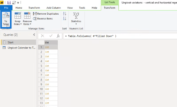
To do that, let’s first convert the list back into a table by clicking the To Table button in the upper left corner.
Then add an index column next to it.
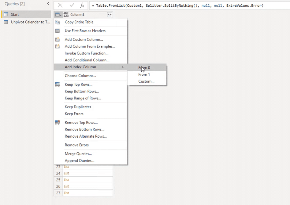
The next thing we’re going to do is to add another column next to the index column. This column should help us determine which values on Column1 contain the date values. Let’s name this column Index2.
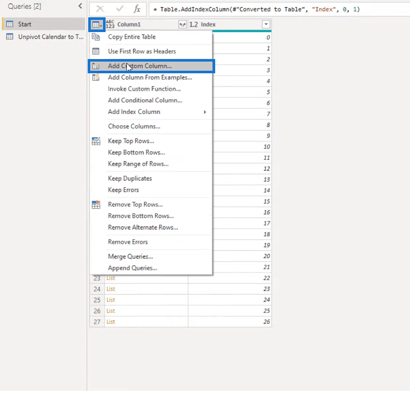
To do that, we’re going to incorporate a formula in Index2, which returns the index value of Column1 if it contains a date.
We’re going to use the IF function, and then reference Column1. The brackets will serve as the operator; adding 0 in between these brackets means we get the first value from the list; then we determine if it is a date. If it is, I want the formula to return the index number; if it is not, I don’t want it to return any value at all.
Since the first value in Column1 contains a date, the first value in Index2 should contain its index number 0. Also, since the second value in Column1 does not contain a date, then the second value in Index2 should only contain a null value.
This is how I’ve set up the formula for Index2. Just make sure that there are no syntax errors in your formula.
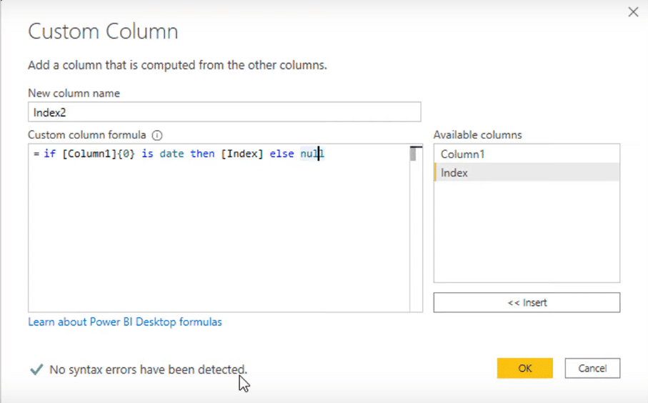
After doing that, our Index2 column should now have the index of the values in Column1 that contains the date. It will also include some null values as a result of the formula that we’ve set up.
Determining Which Values Belong In The Table
Now, these index values inside Index2 indicate the starts and ends of the separate tables that we have. That is, 0 marks the start of the first table, 7 marks the end of the first table, and the start of the second table, and so on.
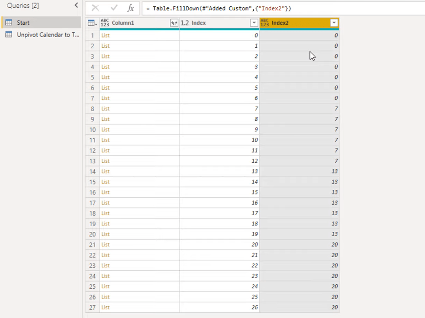
To help us identify which values in Column1 belong in the same table, let’s apply a fill down action in our new column.

After performing the action, the null values should now be replaced by zeros, sevens, thirteens, and twenties. These numbers indicate that they belong in the same table. That is, the zeros form one table, the sevens form another table, and so on.
Grouping the Data For A Proper Tabular Format
Since we already know which values in Column1 belong in the same table, let’s now group them together. To do that, we will be using the Group By operation.

By doing that, we now end up with only 4 values in our Index2 column. Notice that another column named Count is beside our Index2 column. This column counts the number of rows in each of our values in the Index2 column.
However, this isn’t really what we want to do. What we need to do is form a new table using the columns we have.
To do that, we’re going to use the Table.FromColumns operation, reference the column that contains our list values which is Column1, and then change the return type to a table.

It is important to ensure that we’ve referenced the correct column in our formula. Check if Column1 really contains the lists values.
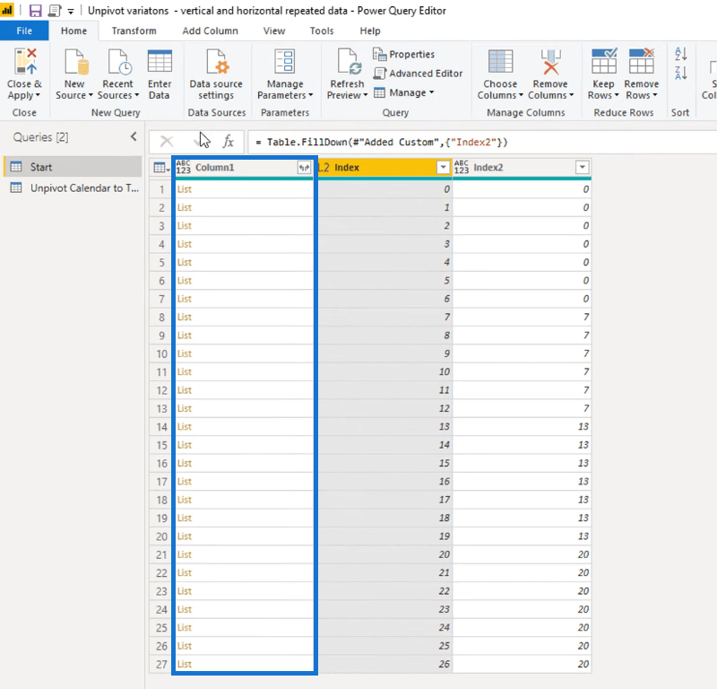
This stitches all of the values in Column1 with an Index2 value of 0 into one table, the ones with the Index2 value of 7 into another table, and so on.
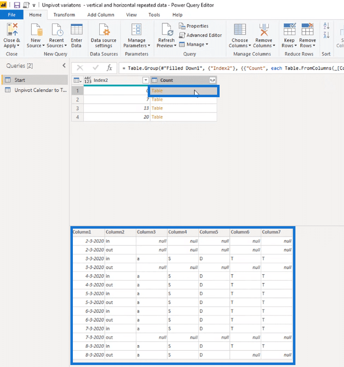
We checked every record to value 0, then retrieved the list value from Column1. Finally, we stitched up those lists to form a single table using this M code.

We grabbed the first 7 columns and stitched them into a single table, grabbed the next few columns, stitched them to another table, and so on.

Appending The Separate Tables
Now that we’ve already grouped them together, let’s try to append all the tables up by adding another step. Again, let’s press the fx button to add a new formula.
The Table.Combine operation merges a list of tables, and then creates one single table out of them. Here, we’re going to reference the column that contains our list of tables, which is the Count column.

We now have a table where all the nested tables are appended back into one big single table.
After appending all the tables up, we can now perform the last few steps in transforming our data into a proper tabular format. Select the first two columns of your table and then click the Unpivot Other Columns button in the Transform tab.

After that, remove the attribute column since we don’t really need it. Go to Choose Columns, then deselect the attribute column.
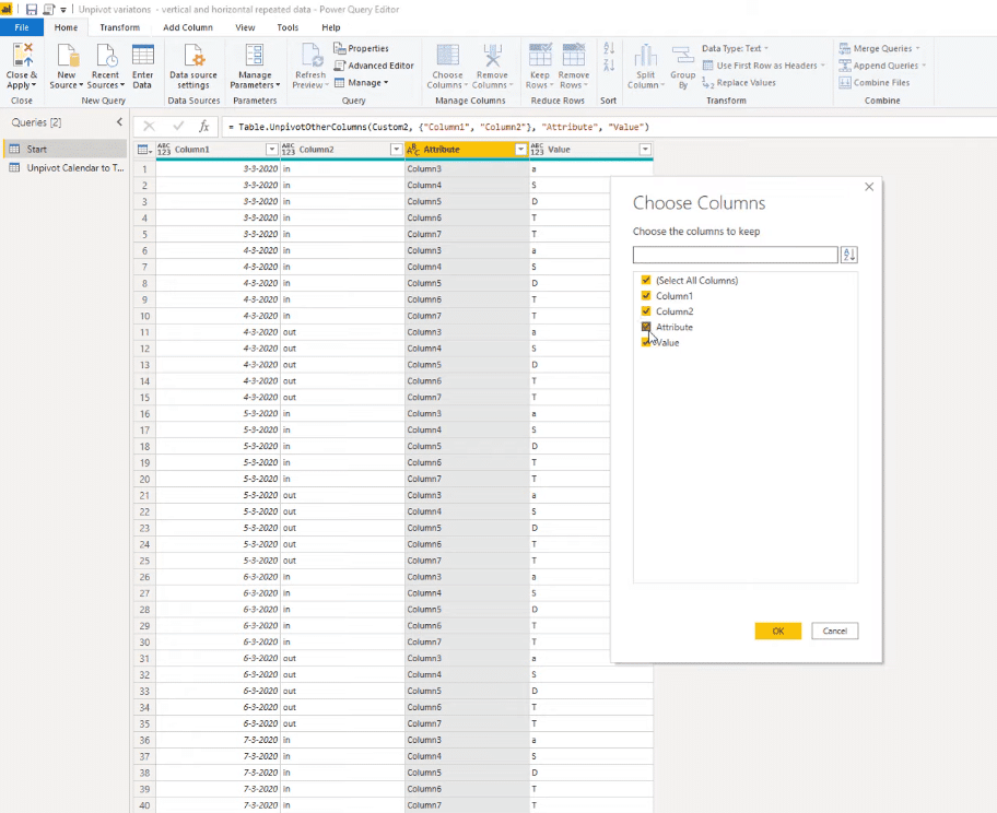
Then finally, set the correct types of all the columns and label them properly.
Double click the column header of each column to change their name accordingly.
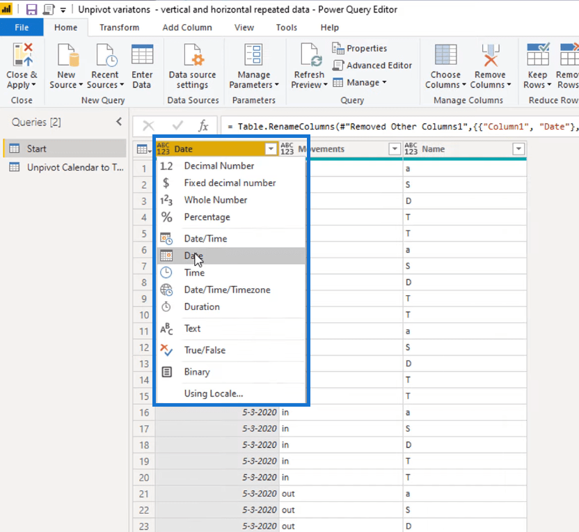
For the first column, change its type to date since it contains our date values.
Then, select the second and third column, and set their types to text.
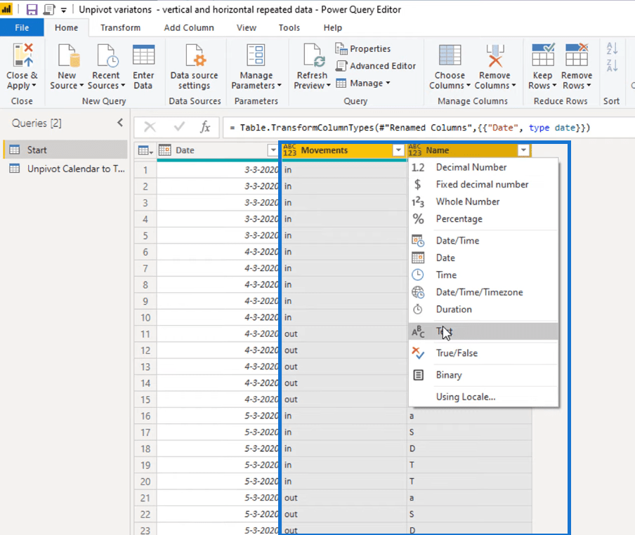
All done! This is what our proper tabular format should look like.
***** Related Links*****
How To Create Automated & Dynamic Power BI Reports
Create Unique Table Template Designs Within Power BI – Power BI & Financial Reporting
Custom Conditional Formatting For Power BI Tables
Conclusion
In this tutorial, we transformed some data, which was presented in a calendar type layout, into a proper tabular format. We first cleaned our data, broke it into smaller tables, grouped the tables that belong together, and then appended them all up in the end.
This tutorial offers you a lot of knowledge on how to properly model your data for easier analysis.
Understanding the concepts that were used here is very important since they can also be applied in a lot of other ways.
If the concepts are still not clear to you, checking the links below might help you.
Enjoy working through this one!
Melissa


