In this tutorial, I’m going to run through some advanced analytics techniques within Power BI and the DAX formula language that I call secondary table logic. You may watch the full video of this tutorial at the bottom of this blog.
Sometimes when using Power BI for your analytics, you’ll want to find or discover interesting insights, but the current data you’re working with may not allow you to extract such insights.
Which is why sometimes it’s crucial to create secondary tables to bring in such information to your core data model.

I show from start to finish how you need to think analytically about utilizing these tables, but then also how to implement them in a really practical way.
We learn better by doing, and so I’ll take you through a practical example of how you can go about doing this on your own. I’ll demonstrate how you can bring in various information or insights to your data analysis that really showcase things in a much more effective way.
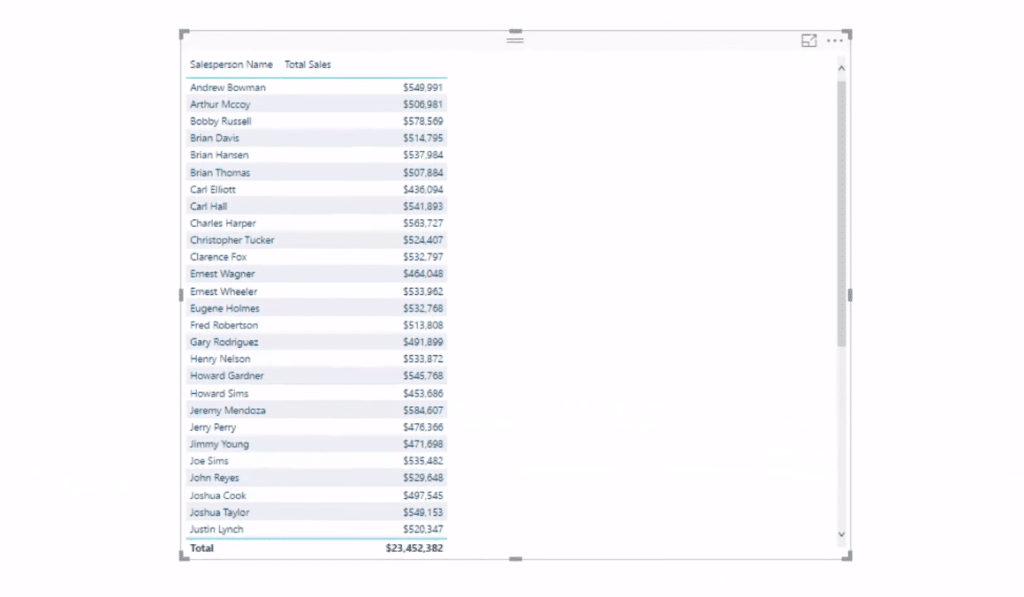
So here we work out the total sales of our salespeople in the last 60 days. And then based on that, we will dynamically classify them as good, mid-range, or bottom salespeople.
As we go through time, we can look back in the last 60 days and see which salespeople at any 60-day period are selling really well.
Branching Out For Secondary Table Logic
Before we dive into creating the secondary table logic, let’s go through the calculations involved in achieving this.
This example here is static in terms of the built-in demo data set, so I had to create a formula that retrieves the last date of my sales table.
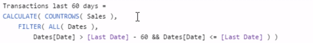
I specifically intend it that way for this demonstration, but you can have it in another way in your own data sets that it would be updating every day. Here’s the formula I created to get the Last Date.


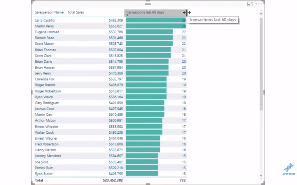
From this, we can then feed this formula into our calculation, Transactions Last 60 Days. In this calculation, we go CALCULATE COUNTROWS of the Sales table. Then, we open the dynamic 60-day window by using FILTER ALL Dates that iterates through the Dates table, which then gives us the results we are looking for.
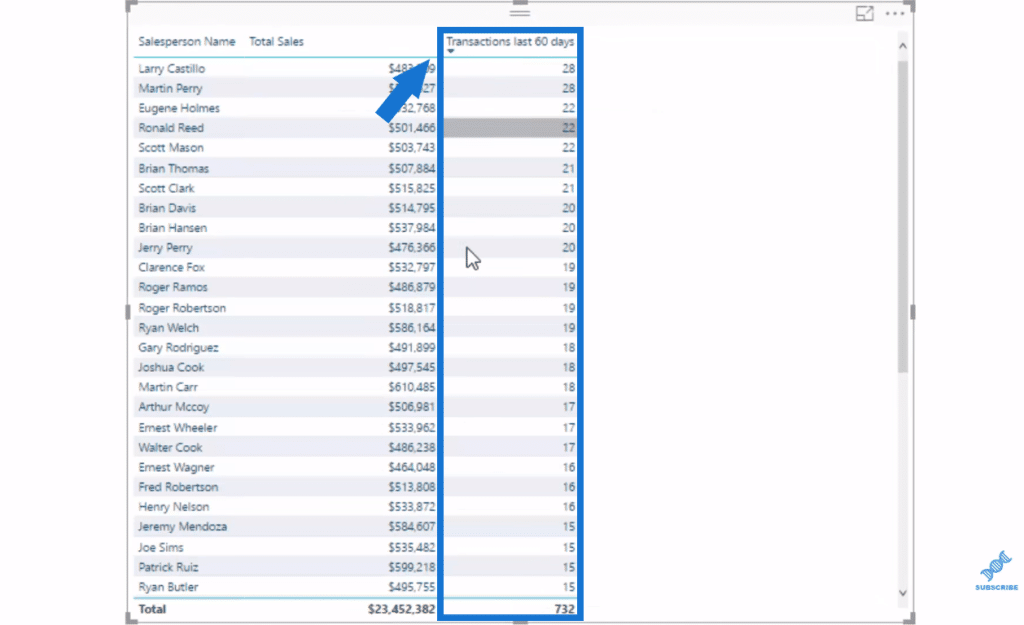
This is going to show us the total sales that any sales person has made in the last 60 days on a rolling basis, as we move through time. As we filter this, we can see our worst and best salespeople.
We can also make this look more visually appealing by using some Data Bars. We go Conditional formatting,
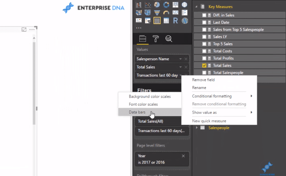
then change it up a little bit with some colors.
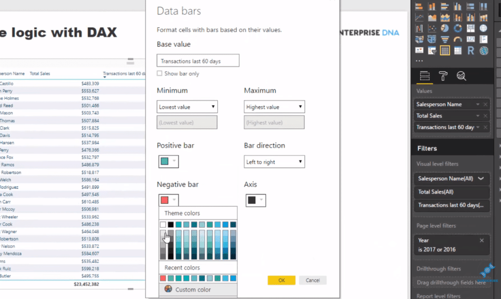
Now we can see clearly our top sales people based on the last 60 days in this data set.
Now this is where the secondary table logic comes in. We’ll group these salespeople based on how many products they sell.
This insight will help us manage our people well, and make better decisions in terms of giving rewards or perhaps even firing those who are not performing at all.
Creating The Secondary Table
A secondary table logic is necessary here because this is a dynamic calculation. We can’t put this into the lookup table. We need to be able to iterate through the numbers into the logic in a secondary table to then group these people.
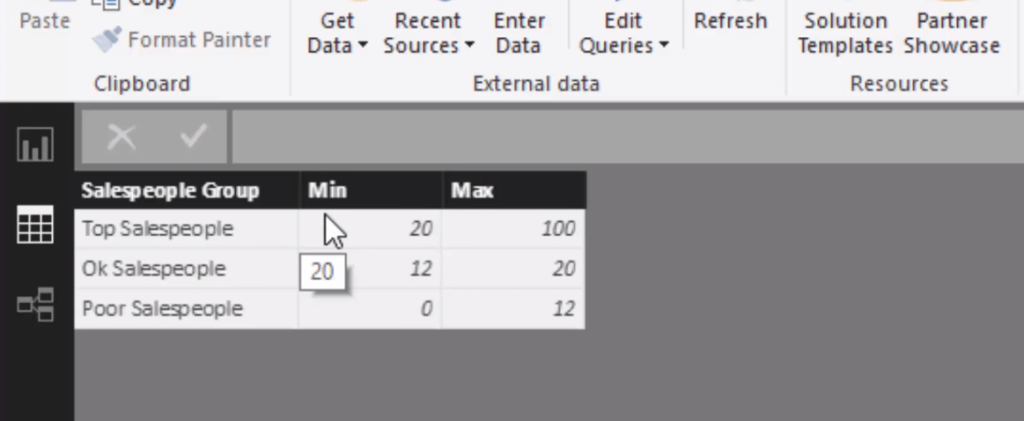
So to create another table, we go Enter Data, then type in the title and the columns.
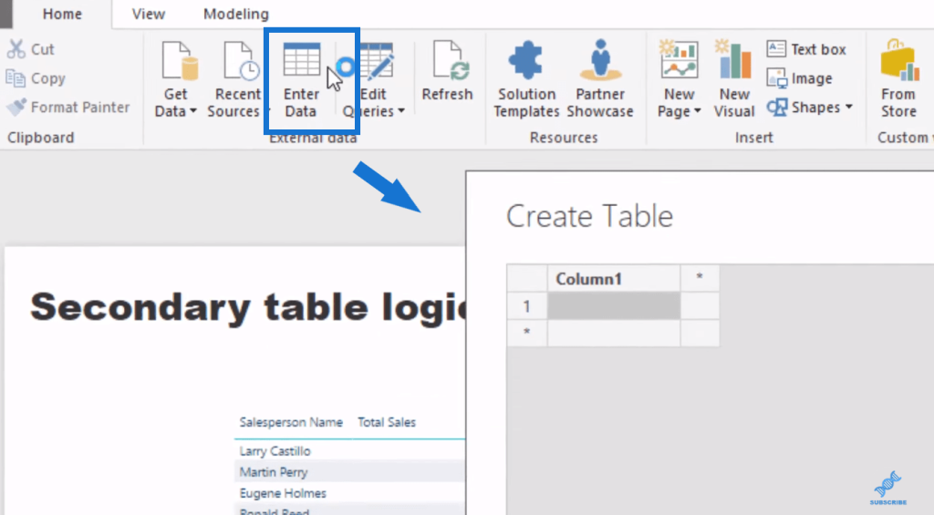
We create our Min and our Max, and then put in the values that we intend to have. Then, we click on Load.
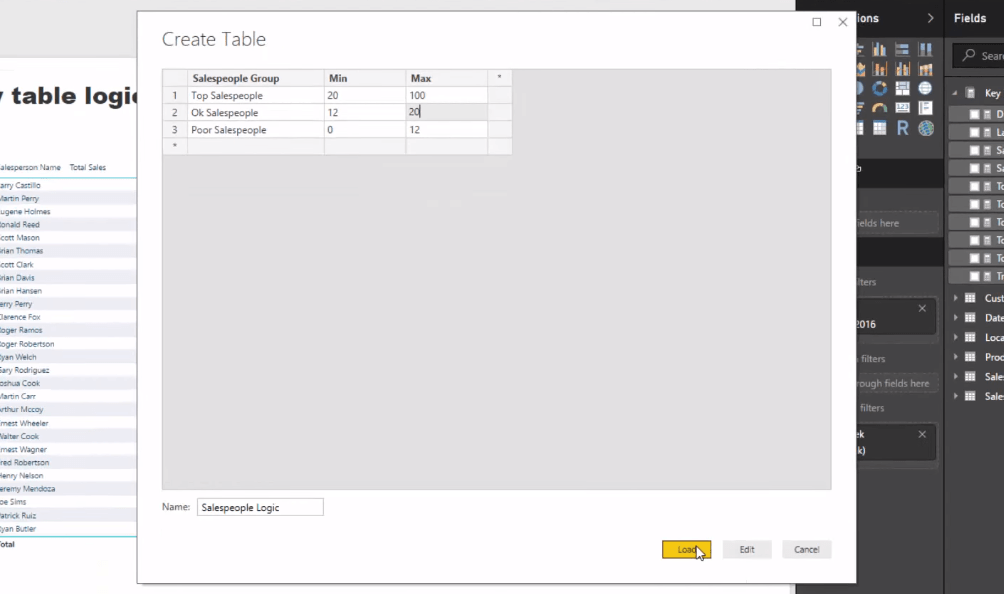
Once that’s loaded up, we’ll have it inside our model. Note that a secondary table has no relationship with our data model. It only sits out here and we don’t connect it to anything because we don’t need to.
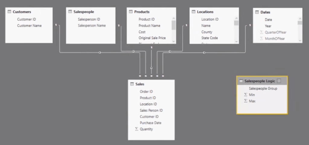
This is the table we need to iterate through. This means that for each sales person and the result we got from our Transaction Last 60 Days, we’ll determine which group they belong based on our Min and Max here.
So now we need to write a formula that would enable us to work out what that is.
Using Secondary Table Logic To Extract Insights
To extract these insights, we need to create a new measure first. We’re going to be returning a text value here because we’ll be putting these people into a group.
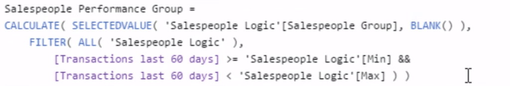
Let’s call this formula Salespeople Performance Group. We utilize the function CALCULATE to SELECTEDVALUE, which is our secondary table logic, where it will find and return one text value (top, OK, poor). We put an alternative result (BLANK) just in case.

Then, on the next line is where we put our secondary table logic. And we use the FILTER function, as it iterates through ALL our Salespeople Logic.
With this logic, we will find out the group that a particular sales person is in, and that group will be dynamic because this measure is dynamic. And so if we bring this into our table, then we’ll now see the results.
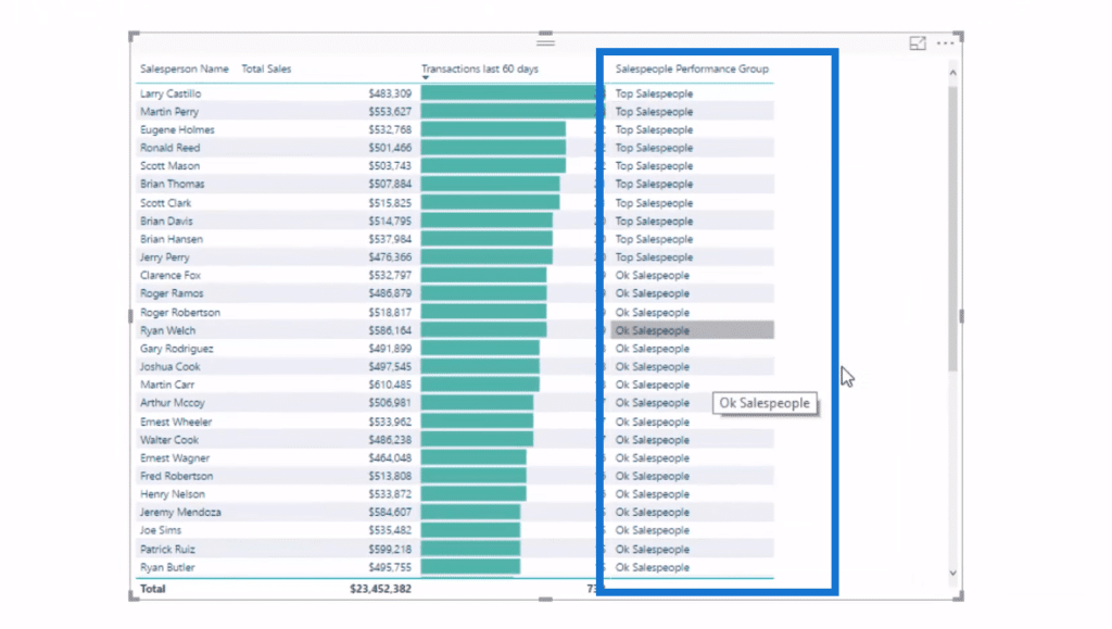
We grabbed a particular figure from another table, which I call a secondary table, and then brought it in via measures into our model.
***** Related Links *****
How To Evaluate Clusters In Your Data Using DAX Technique In Power BI
Use DAX To Segment & Group Data In Power BI
Group Customers Dynamically By Their Ranking w/RANKX In Power BI
Conclusion
This is the power of advanced analytics in Power BI. By utilizing secondary table logic, we don’t need those intermediary calculations. The formula is doing all the hard work for us.
These are all the tips you need to be able to grasp this unique concept in Power BI. These techniques are actually quite unique to Enterprise DNA and to some of the best practice development that we’re completing.
It is only after you read this blog and watch the video below that you’ll get to understand exactly what I mean. So go ahead and review the video. I can promise there is a lot to learn.
Your mind will expand exponentially in terms of the analysis and information that you can get into your reports.
Good luck!
Sam