In this tutorial, we’re going to cover the difference on how data indexing works in a relational database versus in Vertipaq.
Relational databases store the data on a row by row basis. On the other hand, Vertipaq does it column by column.
Let’s see how these two ways of storing and indexing data could impact your report development process especially when running your queries.
Data Indexing Per Row
Storing the data row by row is the traditional way of storing data. However, this process takes more time, which will impact your query’s performance.
Let’s say we have a table that contains the Brand, Color, Gender, Quantity and Net Price.
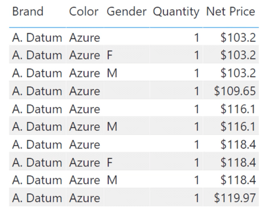
If we store everything in this table in a database, then it will store the data in a row by row basis. That’s why the traditional data storage structure is also called as row store.
First, in the same line, it will store the column headers found on the first row — Brand, Color, Gender, Quantity and Net Price. Then it moves on to the next line to store the first items under each column — A. Datum, Azure, a blank, 1, and 103.2. This continues row by row.

So how are we going to compute for the SUM of the Quantity using this data indexing method?
First, it starts with the first row, which contains the column headers. Then, it jumps into the next line and skips through the other pieces of data until it gets to the first quantity it sees, which is 1. Then it jumps from line to line, running through all the data each row contains and gathers all the quantities is finds.
Once it has set aside all the quantities from each row, that’s the only time that the calculation is completed.
You can probably imagine how tedious the process is if you’re preparing a Power BI report that uses a DirectQuery connection to a SQL data source. In this case, analysis services is going to convert the DAX code into the SQL language, then start going through the data structure row by row.
Data Indexing Per Column
To avoid the lengthy process involved, you have the option to store the data on a column by column basis through Vertipaq when you choose import mode.
When you use column store instead of row store, the Brand, Color, Gender, Quantity and Net Price will each be stored in different data structures.
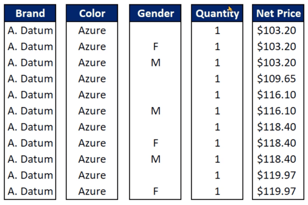
Let’s say we want to get the SUM of the values in the Quantity column. There won’t be any need to pass through the Brand, Color, and other pieces of data outside the Quantity column. In a single scan, it reads the entire Quantity column from top to bottom and sums up all the values.
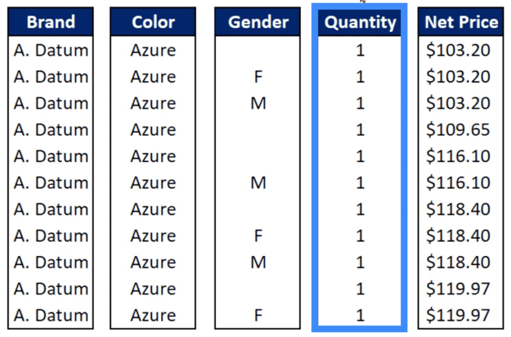
Because of this, the queries will be executed more quickly as compared to doing it from left to right.
Comparing Execution Time In Simple Queries
To really see the huge difference between row store and column store, let’s do some test queries in both SQL and Vertipaq. The execution time should tell us how fast one process is compared to the other.
Let’s start with a simple query in SQL. We’re going to compute for the SUM of the Quantity column in the Sales table.
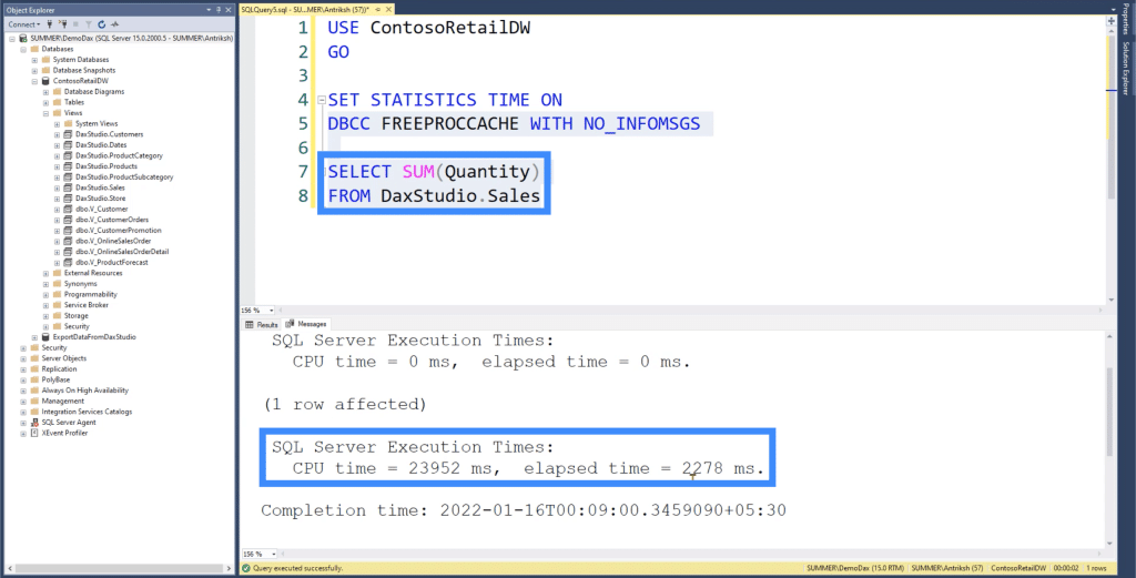
As you can see, the total execution time is 2.2 seconds.
Now, let’s go to DAX Studio and use the EVALUATE function to execute the same query. We need to turn on the server timings and wait for the trace to complete.
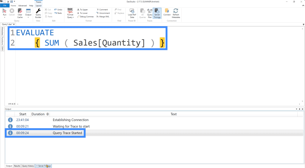
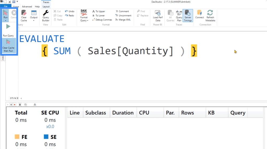
We also need to make sure that the “Clear Cache then Run” option is selected when we run the query.
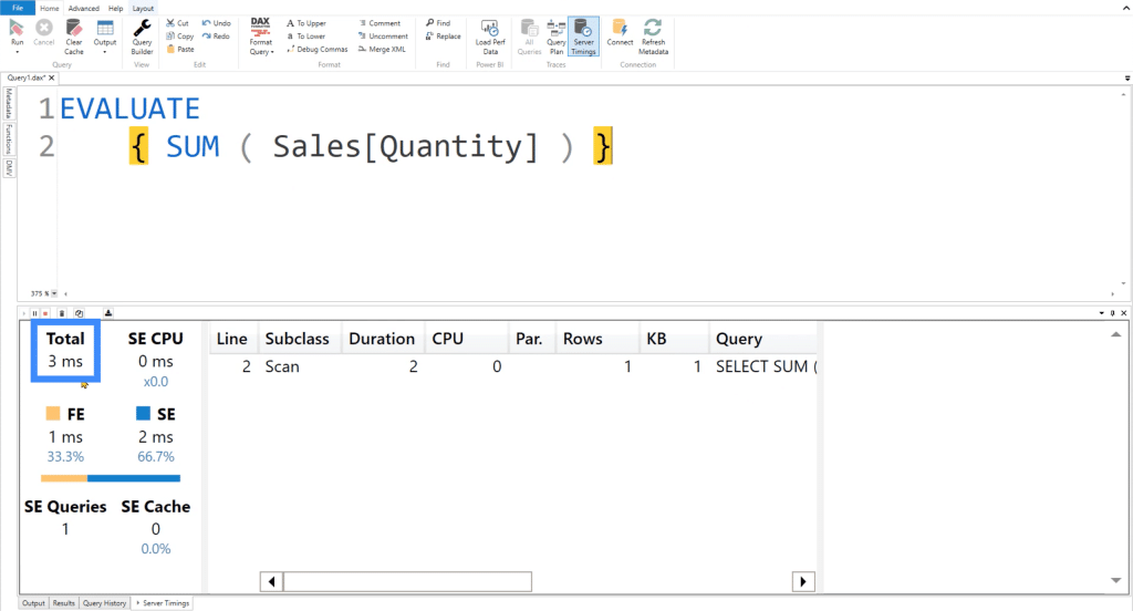
Once the query is executed, you’ll see that it only takes 3 milliseconds to complete the same query we did in SQL earlier.
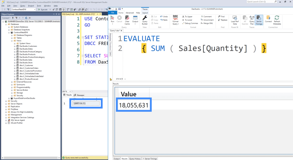
The results set should also match for both SQL and DAX Studio. If we put them side by side, you can see that we are returning the same value.
You can try running the query a few more times to see how consistent the execution time is.
Comparing Execution Time In More Complicated Queries
This time, let’s compare the execution time when we’re running more complicated queries.
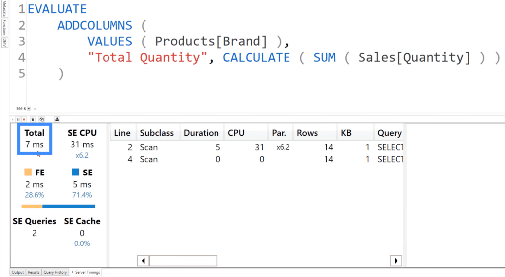
Let’s say we want to identify the SUM of Sales Quantity for each brand. To do this, we can use ADDCOLUMNS over the VALUES of each Product’s Brand. In the low context, we’ll also create a new table called Total Quantity where we’re going to CALCULATE for the SUM of the Sales Quantity.

If we run this code, you can see that the total execution time is 7 milliseconds.
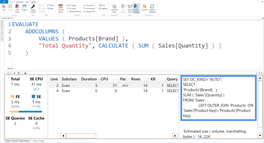
In the background, this code is actually running two queries. The first one takes the Brand column from the Products table, then executes a LEFT OUTER JOIN on the Product Key columns from both the Sales column and the Products column.
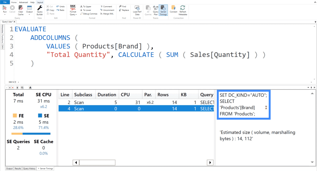
The second query simply retrieves the Brand column from the Products table.
If I go to the results screen, you can see that the Total Quantity measure has been split based on each Brand.

Now let’s go to the SQL server and write the same query.
We’ll push the DaxStudio Sales table to the next line, referencing the Sales table AS S. Then, we’re also going to execute a LEFT JOIN in the DaxStudio Products table referenced AS P, with the S.Product Key equal to the P.Product Key. We’re also going to use P.Brand with the SUM of the Quantity and Total Quantity in the SELECT statement. Finally, we’re going to use GROUPBY for P.brand.
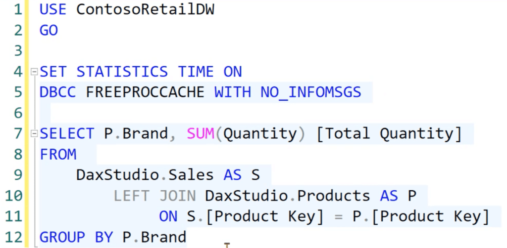
Once we run this code, we’ll get a table that contains the Total Quantity segregated by each Brand, which is the same thing that we previously got in Vertipaq.

As for the total execution time, it remains much slower at 2.5 seconds.

***** Related Links *****
DAX For Power BI: Optimizing Using Formula Engines in DAX Studio
DAX Query Optimization Techniques And Lessons
Query Performance And DAX Studio Setup
Conclusion
It’s evident how fast the column store through Vertipaq really is in comparison to the row store in a SQL database. This shows the importance of really getting to know the way data indexing works through different platforms.
It may seem like a small sacrifice at first if you still choose to go for the 2.5 seconds that the row store runs your query as compared to 7 milliseconds. But we all run several queries when we create our reports and all of those execution times will add up, impacting productivity and user experience in the long run.
Enterprise DNA Experts

