In this post, we’re going to show you how to use the Chi-square test in Excel to compare variables. You can watch the full video of this tutorial at the bottom of this blog.
The Chi-square test of independence has two categorical variables. We will find out if there’s any relationship between those variables.
We will be using the hypothesis testing framework. In case you are not familiar with this, check out the Advancing Into Analytics book. This is an advanced analytics technique using Excel, R, and Python.
For our demo, we will be using a housing data set in Excel. We need to get the actual values using the pivot table and then compare this to the expected values using formulas.
We will also check the 95% significance level and if there’s a relationship between the air conditioning and the preferred area.
Using Chi-square Test In Excel To Compare Variables
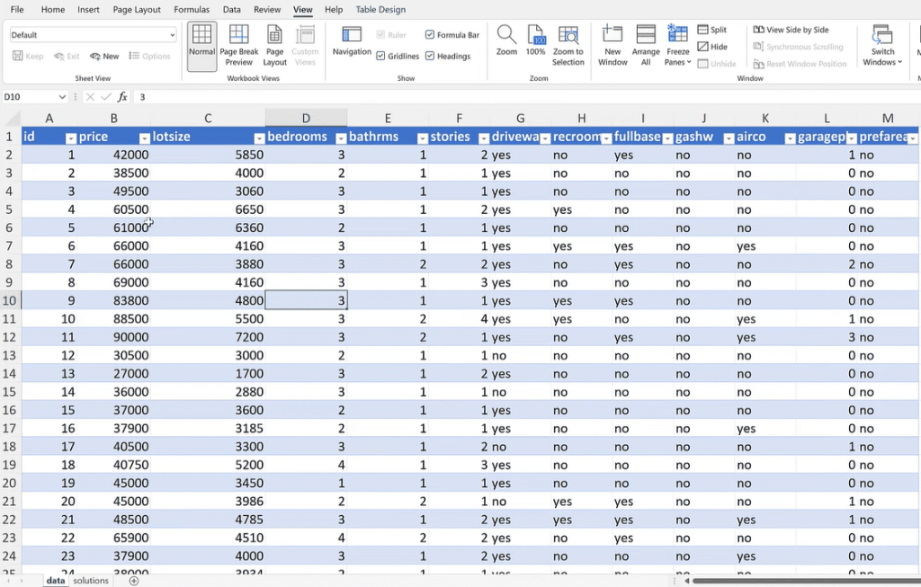
Let’s jump into Excel. These are the housing prices that came from the Journal of Applied Econometrics.
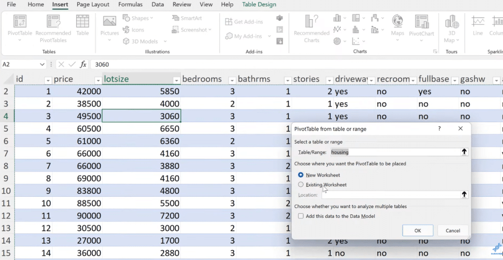
Insert a Pivot table, then click OK to use an index column to count observations.
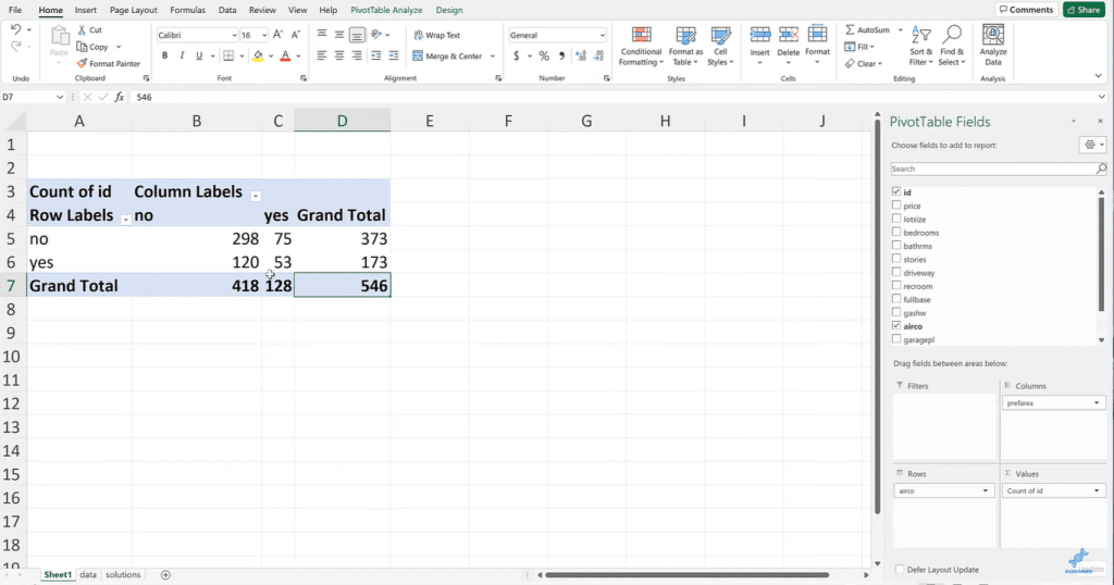
From the Pivot table fields, drag ‘id‘ into Values section. Select Count from the Value Field Settings since these are all unique values.
Next is to drag ‘prefarea‘ into Columns and then drag ‘airco‘ into Rows sections to see the actual values.
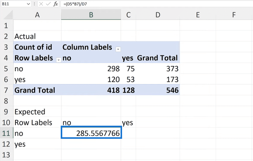
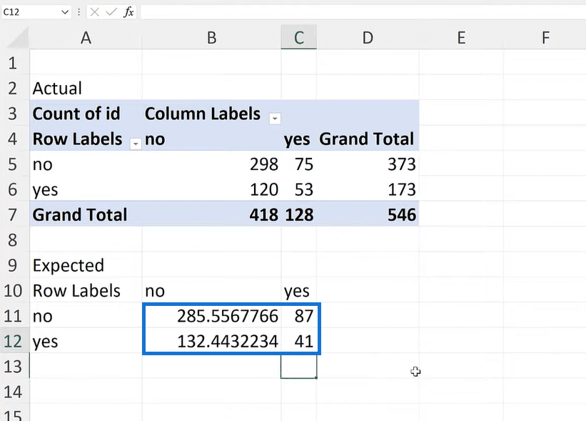
We have a total of 546 observations. The 298 are neither air conditioning nor preferred area, while 53 are both and so on.
Let’s create two tables and label them as Actual and Expected.
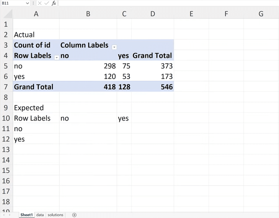
To get the expected values for neither air conditioning nor preferred area, multiply D5 by B7, then divide it by D7.
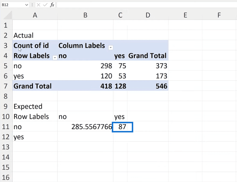
Next is to get the expected value of either the air conditioning or preferred area, multiply D5 by C7, then divide it by D7.
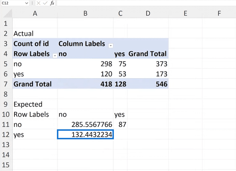
Now for the expected value of either the preferred area or air conditioning, multiply D6 by B7, then divide it by D7.
Lastly, let’s compute the expected value of both air conditioning and the preferred area. Multiply D6 by C7, then divide it by D7.
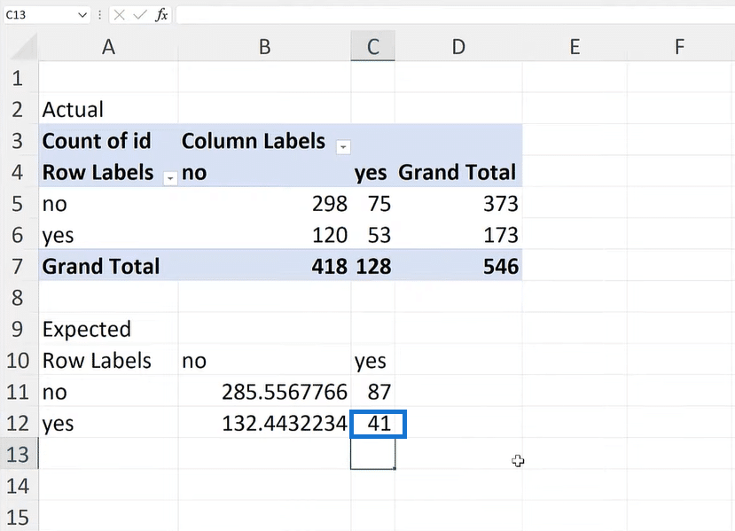
Highlight the range of the expected values to find out the sum, which should be 546.
Now we will find the relationship between the actual and expected values. Let’s check if they tend to move together in a way.
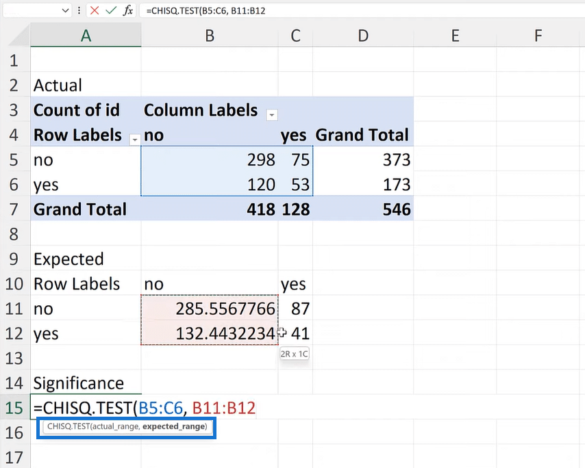
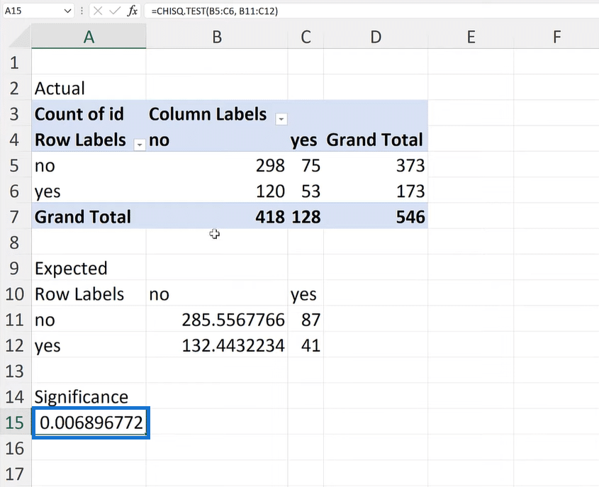
To find the Significance, type =CHISQ.TEST. Highlight the range of the actual values, add a comma, then highlight the range of the expected values to get the p-value.
Based on the result, this is a slight random chance. There seems to be some relationship between the preferred area variable and the air conditioning variable.
***** Related Links *****
Merge Queries Using Anti Join In Excel With Power Query
Count Distinct Values In Excel: Classic To Modern Approaches
Proportion And Frequency Tables In Excel
Conclusion
The Chi-square test is a common technique that helps us know the difference by category, and is a good example of A/B testing.
Another thing to remember is that the observations need to be independent. Based on our example, we are looking at two binary variables, a specific type of categorical variable.
Lastly, let’s be aware that it can get tricky when we have a lot of categories.
I hope this is something that you can use for A/B testing, whether in Excel or Python.
All the best,
George


