
New to Excel or just forgotten how to merge two columns?
In Microsoft Excel, merging columns is a straightforward process that allows you to bring together data from different sources into a single, easily accessible location. Period.
To merge two columns in Excel, you can use the CONCATENATE function, the & operator, or the TEXTJOIN function. For a simple merge, place =A1 & ” ” & B1 in a new column, where A1 and B1 are the first cells of your columns to be merged; this formula combines the content of A1 and B1 with a space in between.

This article will guide you through 6 great ways to merge columns in Excel. Each method will be followed by examples to help you better understand the concepts.
Why 6? Well everyone has preferences and slightly different situations, so please go through them all and pick which works best for your use case.
Time to Excel!

6 Methods to Merge Two Columns in Excel
In this section, we will go over 6 methods to merge two columns in Excel.
The 6 methods are:
Using the CONCATENATE Function
Using the Ampersand (&) Operator
Using the TEXTJOIN Function
Using the CONCAT Function
Using Power Query
Using Flash Fill

1. How to Merge Two Columns Using The CONCATENATE Function
The CONCATENATE function allows you to join the contents of two or more cells, with the option to include text or other characters as separators.

To merge columns using the CONCATENATE function, follow the steps below:
Step 1: Select the Cell for Merged Data
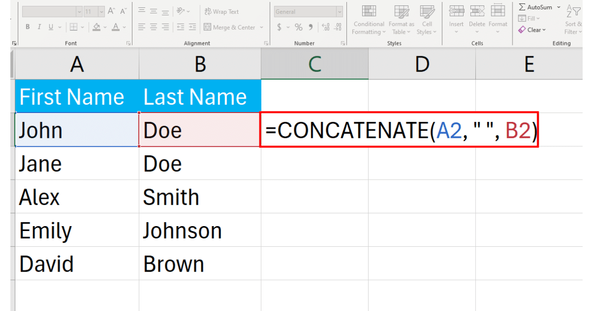
Suppose we have a list of first names in one column and last names in another.

Click on the cell where you want the merged data to appear. In our case, this would be cell C2.
Step 2: Use the CONCATENATE Function
In the selected cell, type an equal sign (=) to start the formula, followed by the CONCATENATE function and opening parenthesis.
For example, if you want to merge the first name in cell A2 and the last name in cell B2, you would type:
=CONCATENATE(A2, " ", B2)In Excel, the formula looks like the following:
Step 3: Press Enter
Press Enter on your keyboard, and the contents of the two cells will be merged into a single cell.
You can now see the full name in cell C2.
To merge more rows, you can simply drag the fill handle down in the merged cell, and it will automatically show the combined data in a single column.

2. How to Merge Two Columns Using The Ampersand (&) Operator
The Ampersand is a special character that is used to concatenate, or join, the contents of two or more cells.
This operator can be useful for merging columns with text, numbers, or a combination of both.
To merge columns using the Ampersand operator, follow the steps below:
Step 1: Select the Cell for Merged Data
Click on the cell where you want the merged data to appear.
In our case, this would be cell C2.
Step 2: Use the Ampersand Operator
In the selected cell, type an equal sign (=) to start the formula, followed by the first cell reference containing the data you want to merge.

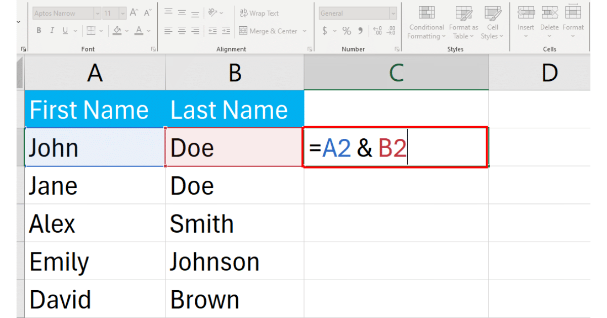
The formula in cell C2 would look like this:
=A2 & B2In Excel, the formula to formula to combine columns will look like the following:
Step 3: Press Enter
Press Enter on your keyboard, and the contents of the two cells will be merged into a single cell. You can now see the full name in cell C2.
To merge more rows, you can simply drag the fill handle down in the merged cell, and it will automatically merge the corresponding rows.
3. How to Merge Two Columns Using The TextJoin Function
To merge two or more columns using the TEXTJOIN function in Excel, follow the steps given below:
Step 1: Select the Cell for Merged Data
Click on the cell where you want the merged data to appear. In our case, this would be cell C2.
Step 2: Use the TEXTJOIN Function
In the selected cell, type the TEXTJOIN function formula. This function requires specifying a delimiter, whether to ignore empty cells, and the cells to merge.
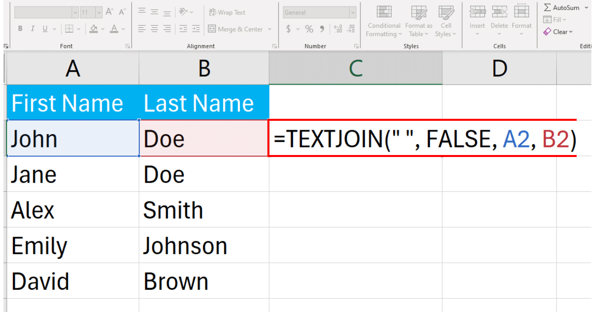
For merging without ignoring empty cells and using a space as a delimiter, the formula in cell C2 would look like this:
=TEXTJOIN(” “, FALSE, A2, B2)
This tells Excel to merge the contents of cells A2 and B2, separated by a space.
Step 3: Press Enter
Press Enter on your keyboard. The contents of the two cells will be merged into cell C2.
To apply this to more rows, drag the fill handle down from cell C2. Excel will automatically apply the formula to the adjacent cells, merging the corresponding rows from the two columns with your specified settings.

4. How to Merge Two Columns Using The CONCAT Function
The CONCAT function is a straightforward approach that combines the contents of two or more cells directly.
To merge two columns using the CONCAT function in Excel, follow these steps:
Step 1: Select the Cell for Merged Data
Click on the cell in an Excel worksheet where you want the merged data to appear.
In our case, this would be cell C2.
Step 2: Use the CONCAT Function
In the selected cell, type the CONCAT function formula. This function concatenates the contents of the specified cells exactly as they are.
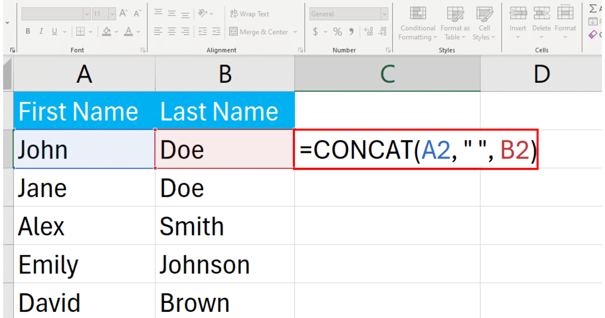
The formula would be:
=CONCAT(A2, B2)If you wish to include a space or another separator between the merged contents, you would manually insert it like this:
=CONCAT(A2, " ", B2)This quotation marks ensures that there’s a space between the first and last names.
In Excel, the formula to merge data looks like the following:

Step 3: Press Enter
Press Enter, and the contents of the two cells (A2 and B2) will be merged into cell C2 as specified.
Drag the fill handle down from the corner of cell C2.
Excel will automatically replicate the formula for the adjacent cells, merging the corresponding rows from the two columns as per your formula.

5. How to Merge Two Columns Using Power Query
Merging two Excel columns using Power Query is a powerful method for combining data, especially when dealing with large datasets or when you need to perform additional transformations.
Follow the steps given below to merge two columns using Power Query:
Step 1: Import Data into Power Query
First, ensure your data is in a range or table format. Click anywhere inside your dataset.
Go to the Data tab on the Ribbon, and click From Table/Range in the Get & Transform Data group. If your data isn’t already in a table, Excel will prompt you to create one.

This will open up the Power Query Editor
Step 2: Merge Columns in Power Query
In the Power Query Editor, select the two columns you want to merge. You can do this by clicking one column, then holding the Ctrl key and clicking the second column.
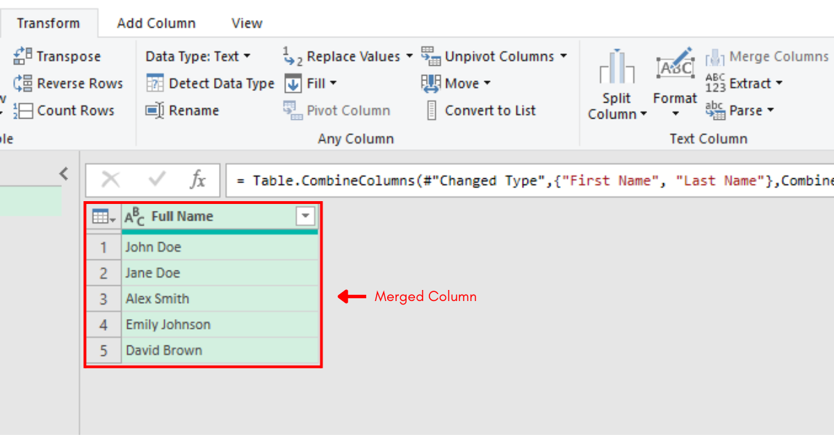
With both columns selected, navigate to the Transform tab and click Merge Columns.
In the Merge Columns dialog, you can choose a separator (such as space, comma, etc.), and provide a new name for the merged column.
Click OK after configuring.
Power Query will merge the two columns into a single column.
6. How to Merge Two Columns Using Flash Fill
Merging two columns using Flash Fill in Excel is a quick and efficient method, especially useful for combining text in a pattern that Excel can recognize.
Follow the steps below to merge two columns using flash fill:
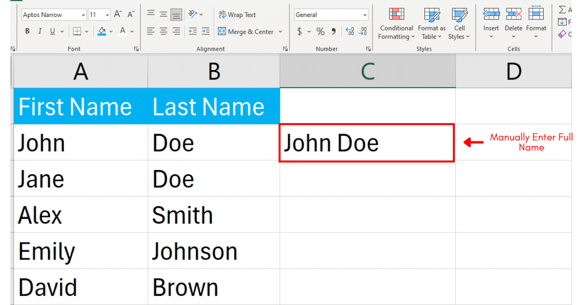
Step 1: Manual Entry
In the cell adjacent to your data, manually enter the merged format you desire from the first row of data.
If you’re combining first names in column A with last names in column B, type the full name as you wish it to appear (e.g., “John Doe”).
Step 2: Activate Flash Fill
Select the entire column, navigate to the Data pane, and click Flash Fill.
Excel will automatically populate the entire column by merging the first and last names columns.

Learn how to count distinct values in Excel by watching the following video:
Final Thoughts
Merging two columns in Excel might seem like a simple task at first glance, but mastering this skill opens up a world of efficiency and clarity in your data management.
So, whether you’re consolidating names, addresses, or any other information, knowing how to blend columns effectively saves you time and prevents the headache of manual data entry errors.
Furthermore, learning these techniques—from the straightforward use of the Ampersand (&) operator and CONCAT function to the more advanced capabilities of Power Query and Flash Fill—equips you with the tools to handle a wide array of data processing tasks.
Remember, It’s about more than just combining text; it’s about refining your workflow, ensuring accuracy, and presenting your data in the most useful way possible.
Happy Excelling!
Frequently Asked Questions
In this section, you will find some frequently asked questions you may have when merging two columns in Excel.
How can I merge multiple columns into a single column in Excel?
To merge multiple columns into a single column in Excel file, you can use the CONCATENATE function.
Simply enter the function as follows: =CONCATENATE(A1, B1, C1), where A1, B1, and C1 are cell references.
The merged cells will be placed into a single cell.
What is the formula for combining two columns in Excel?
The formula for combining two columns in Excel is the CONCATENATE function or the “&” operator. For example, to combine data from cells A1 and B1, you can use either =CONCATENATE(A1, B1) or =A1&B1.
How do I merge columns and keep data in Excel?
To merge columns and keep data in Excel, you can use the CONCATENATE function with a separator. For example, to merge cells A1 and B1 with a space in between, use the formula =CONCATENATE(A1, “ “, B1).
What is the best way to merge columns without losing data?
The best way for merging cells without losing data is to use the CONCATENATE function or the “&” operator.
These methods allow you to combine the contents of multiple cells into a single cell while preserving the original data.
How can I merge columns in Excel and separate them with a comma?
To merge columns in Excel and separate them with a comma, use the CONCATENATE function with a comma enclosed in double quotes.
For example, to merge cells A1 and B1 with a comma in between, use the formula =CONCATENATE(A1, “, “, B1).


