
In Excel, one useful thing you can learn to do is to count how many cells have certain words or specific words in them.
In fact, this is something every Excel user should know how to do.

It basically, helps you see how often particular words or phrases come up in your data, or just find cells that don’t have numbers.
To count cells with text, you can use this simple formula:
=COUNTIF(range, “Specific text”)
But.
And there is always a but.
There are also other formulas to count cells with text under certain conditions, or even count cells without needing to say exactly what text you’re looking for.
In this article, we’ll show you different ways to count cells with text in Excel. Let’s begin!

What are The Text Values in Excel?
In Excel, text is any combination of characters, such as words, numbers, or symbols, that form text strings.
Text strings can be used in formulas, cell contents, or other spreadsheet elements. Understanding how to work with text, characters, and substrings can significantly improve your Excel skills and enhance your data management capabilities.

A text string in Excel refers to a sequence of characters, which may include letters, digits, spaces, punctuation marks, and other special symbols.
For instance, “Hello, World!” is a text string containing words, spaces, and special punctuation. Text strings can be used in Excel functions to manipulate, analyze, or return specific text values.
When dealing with text values in Excel, it is essential to recognize that they are different from numerical values.
Even though you may see numbers within a text string, the cell containing this text will not be treated as a number for calculations or other numerical operations.
Instead, Excel reads and processes these numbers as characters within the text value.
A substring is a part of a text string, typically consisting of consecutive characters within the larger text. Substrings are useful when you want to extract or analyze specific parts of textual data in Excel.
For example, you might want to get the first word of a sentence, the domain of an email address, or specific parts of a product code.
In summary, using text strings effectively in Excel requires understanding the difference between text and numerical values, and working with substrings.
How to Count Cells with Any Text Value?
In Microsoft Excel, sometimes you need to count cells that contain text within a specific range.
Excel offers various functions to achieve this, such as the COUNTIF and SUMPRODUCT functions. Let’s go through two different methods of counting cells with text.
Method 1: Using the COUNTIF function
To count cells with text in a specific range, you can use the COUNTIF function alongside the asterisk (*) wildcard.
For example, if you want to count text-containing cells in the range B2 to B8, you can apply the following formula:
=COUNTIF(B2:B8, "*")
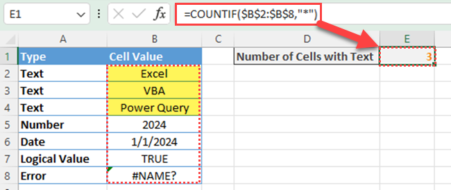
This formula counts only the cells that contain text values. It excludes cells with only numeric values, dates, logical values (true and false values), errors, or empty cells in the specified range.

Remember that Excel counts even a space character as a text character.
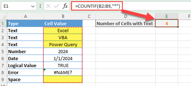
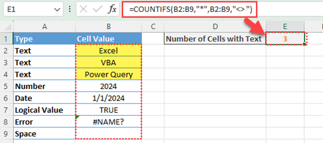
If you want to exclude space characters when counting text values in column B, you can modify the formula as follows.
=COUNTIFS(B2:B9,"*",B2:B9,"<> ")
Method 2: Using SUMPRODUCT and ISTEXT functions
To count text cells, you can also use the SUMPRODUCT and ISTEXT functions together:
=SUMPRODUCT(ISTEXT(B2:B8)*1)
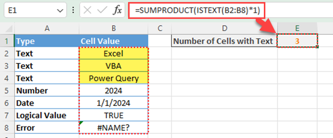
The ISTEXT function checks whether each cell in the range contains text and returns a list of TRUE or FALSE values. If the cell contains a text value, the function returns TRUE. If the cell contains a non-text value such as a numeric value, the function returns FALSE.
By multiplying 1, you can convert TRUE and FALSE values to 1s and 0s.
The SUMPRODUCT function then adds up those TRUE values (converted to 1s) and returns the number of cells containing text.
By leveraging these methods, you can confidently analyze the presence of text in cells within your Excel spreadsheets.
How to Count Cells that Contains a Given Text Value?
To count cells with specific text, you have to modify the COUNTIF argument.
For example, if you want to count cells that contain the word “Excel”, you have to use the below COUNTIF formula.
=COUNTIF(A1:A5, "Excel")
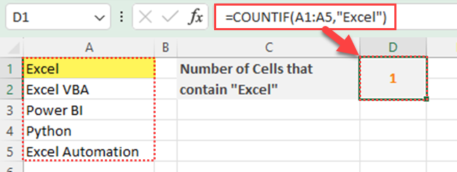
In this example, the formula counts the number of cells that contain only the text “Excel” within the given range.
If you want, you can give a cell reference to the criteria.
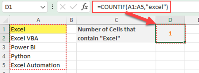
It is important to note that the COUNTIF function is not a case-sensitive function. For example, even if you enter “excel” for the criteria, Excel counts as “Excel”.
How to Count Cells that Contains a Given Exact Text Value (Case Sensitive)?
To count cells containing an exact case-sensitive text value, you can use a combination of Excel’s EXACT function and the SUMPRODUCT function.
If you want to count only cells containing the exact word “Excel” in a case-sensitive manner (not excel, EXCEL etc.), use this formula.
=SUMPRODUCT(EXACT(A1:A6,"Excel")*1)
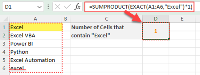
In the formula provided, Excel exclusively counts cells with the text “Excel” and does not include variations like “excel” due to the use of the EXACT function, which is case-sensitive.
How to Count Cells with Partial Text Value?
Sometimes you may want to find how many cells contain a specific text even with partial matches.
In such situations, you have to enter the criteria argument with a wildcard character.
Wildcards help you to do searches and match strings without specifying the exact text. There are several wildcard characters you can use in Excel to achieve this:
- Asterisk (*): Represents any number of characters (including zero characters). For example, text will match any cells containing the word “text” anywhere within the cell.
- Question mark (?): Represents a single character. For example, t?xt will match cells containing “text,” “taxt,” or “t0xt.”
- Tilde (~): This character is used when you want to search for an actual asterisk, question mark, or tilde in the text. To do this, place the tilde before the character you want to search. For instance, ~? will match cells containing a question mark.
For example, if you want to count all the cells that include the word “Excel”, you have to use the below formula.

=COUNTIF(A1:A5,"*Excel*")
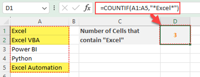
In this example, the formula counts the number of cells that contain the text “Excel” within the given range.
Using these wildcard characters, you can make the COUNTIF function more powerful and flexible.
How to Count Cells Containing Any of the Given Text Values?
Now, let’s say you want to count cells containing any of the given text values. In this case, you can use two or more COUNTIF functions.
For example, if you want to count cells that contain Red or Blue, you can use the below formula.
=COUNTIF(A1:C4,"Red")+COUNTIF(A1:C4,"Blue")
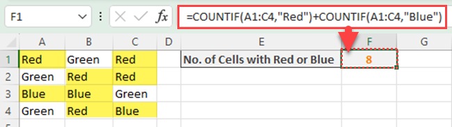
This formula will count the cells that meet either of the specified criteria.
The first COUNTIF function counts cells with the text value “Red”. The second COUNTIF function counts cells with the text value “Blue”. Then, the results are added together.
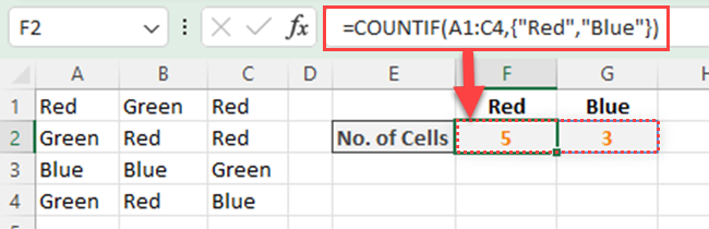
You can count cells with the words “RED” and “Blue” separately by using the COUNTIF function as an array formula in the following way.
=COUNTIF(A1:C4,{"Red","Blue"})
How to Count Cells With Two or More of the Given Text Values?
The COUNTIFS function in Excel is a powerful tool that helps you count cells based on multiple criteria.
It enables you to apply different conditions to your data and provides a count of cells that meet all the specified criteria. The syntax for the COUNTIFS function is as follows:
COUNTIFS(criteria_range1, criteria1, [criteria_range2, criteria2]…)
In this function, criteria_range1 refers to the first range of cells that you want to evaluate, while criteria1 refers to the condition that these cells need to meet. You can add additional criteria with their respective ranges to further filter the cells that will be counted.
For example, if you want to count cells that contain “Excel” and “VBA” you can use the below formula.
=COUNTIFS(A1:A6,"*Excel*",A1:A6,"*VBA*")
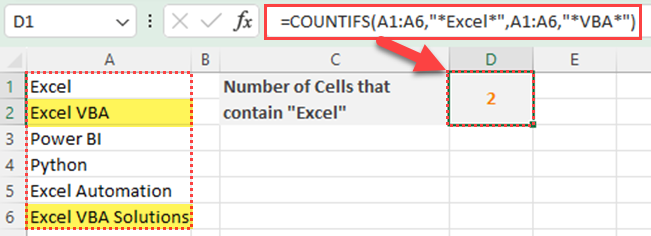
To count cells that include specific text, you can use a combination of the provided text and wildcards as your criteria.
By keeping these features and functionalities in mind, you can effectively leverage the power of Excel’s COUNTIFS function to analyze your data and gain valuable insights.
Final Thoughts
In summary, getting good at counting text cells in Excel gives you lots of ways to work with your data.
Now that you’ve learned a few ways to do it, you can pick the one that works best for you. Whether you like the case-sensitive way with EXACT and SUMPRODUCT, the flexible COUNTIF method, or any other way we talked about, you’ve got tools to make your Excel work easier. So, go ahead and use these tricks to make Excel work better for you.
If you want to learn different approaches on how you can count distinct values in Excel from a more traditional way to a more modern technique, watch the below video.
Frequently Asked Questions
How to count cells containing specific text?
To count cells containing specific text in Excel, use the COUNTIF function with the text you want to count enclosed in quotes and asterisks. For example, =COUNTIF(range,”*text*”). Replace “range” with the cell range you want to search, and “text” with the text you want to count.
What is the method to count non-blank cells?
Counting non-blank cells in Excel can be done using the COUNTA function. Type the formula =COUNTA(range) into a cell and replace “range” with the cell range you wish to evaluate. This function counts the number of cells that contain any value, including text, numbers, and errors, excluding blank cells.
How can I use COUNTIF with multiple criteria?
To use COUNTIF with multiple criteria, you can use the COUNTIFS function. The syntax is =COUNTIFS(criteria_range1, criteria1, criteria_range2, criteria2, …). Replace “criteria_range” with the cell range and “criteria” with the condition. You can include multiple criteria as needed, with each additional criteria_range and criteria pair.
What is the process of counting names in Excel?
You can count names in Excel by using the COUNTIF or COUNTIFS function, depending on whether you want to count a single name or multiple names. For a single name, use =COUNTIF(range,”name”), replacing “range” with the cells you want to search, and “name” with the name you want to count. For multiple names, use the COUNTIFS function, as described in the previous question.
How do you apply COUNTIF on multiple ranges?
To apply COUNTIF on multiple ranges, you can use the SUM function to combine separate COUNTIF functions for each range. The formula would look like this: =SUM(COUNTIF(range1, criteria), COUNTIF(range2, criteria), …). Replace “range” with the cell ranges you want to evaluate and “criteria” with the condition you want to count.
Is there a way to count cells with text in Google Sheets?
Yes, counting cells with text in Google Sheets is similar to Excel. Use the COUNTIF function with an asterisk as the criteria. For example, =COUNTIF(range, “*”). Replace “range” with the cell range you want to search. The asterisk acts as a wildcard, matching any sequence of characters and counting cells containing any text.


")