
Parallel coordinate plots are a useful visualization tool used to show relationships between multiple variables sharing the same numerical data. In Power BI, these plots are created with very simple Python code that you can use and easily create and stylize.
In today’s blog, we will learn how to create multi-variate or parallel coordinate plots using Python. We will walk through the process step-by-step, from preparing the data to customizing the plot for better readability. You can watch the full video of this tutorial at the bottom of this blog.

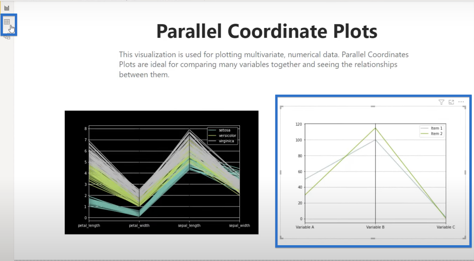
Parallel Coordinate Plots In Python: Sample 1
This is our first plot. It shows our three variables—Variable A, B, and C, and the two lines representing Items 1 and 2.

That means we have two sets of data, one for Item 1 and another for Item 2. And for each dataset, we have our three variables.
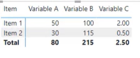
Let’s look at the data to better understand how the plot was structured.
Start by highlighting the graph. Click Data.
A table with very simple data should appear. It was created using the insert table option. We can see that in the columns are Variables A, B, and C for each item that are separated in each row.

We have simple data, but we can turn it into something that is very telling. For instance, in our plot, we can determine that the relationship among the data is quite “low.”
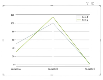
To illustrate, we can compare this plot to our data. Variable B in Item 1 is 100 and 115 in Item 2, as shown in the graph.
We can also identify how the items and variables are related. For example, we can easily see that Variable A is lower than B, and that C is the lowest among the three.
The Plot Python Code
Let’s now proceed with the Python code used for the actual plot.
Start by choosing Python visual from the Visualizations pane.

Highlight our first graph to open the Python script editor.
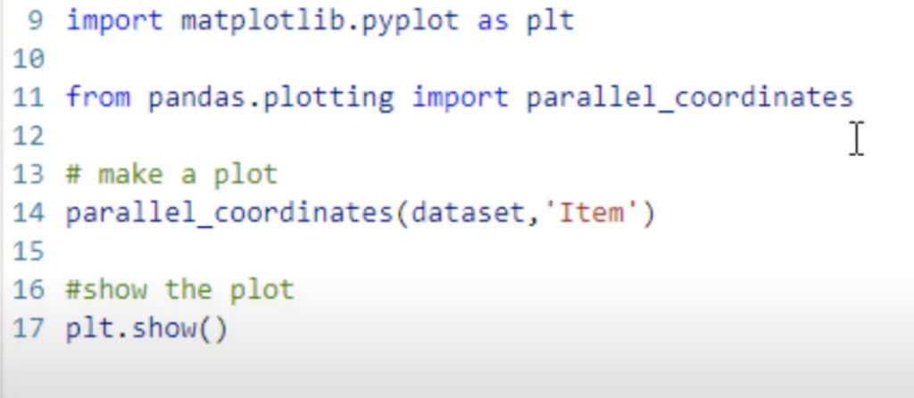
First, we import matplotlib.pyplot and save it as a variable plt.

Then, we bring in the pandas.plotting features. Pandas serves as a data manipulation library in Power BI. It’s primarily used to manipulate data, but it also has plotting features.
Let’s import parallel_coordinates from pandas.plotting. Parallel_coordinates will be the primary function for creating the graph.

Making The Plot In Python
In line 13, we document what we are going to do by writing # make a plot.

We use parallel_coordinates and pass in the dataset.

In line 3, we can see the dataset is created using the pandas.DataFrame ( ) function. Then, we add Item, Variable A, Variable B, and Variable C, which are then reflected in our Values list.
In line 4, the dataset is deduplicated using dataset.drop_duplicates ( ).

We can go to the Visualizations pane to see the Values that we added.

Removing any one of these values will affect our visuals. For instance, if we remove Variable C, the coordinates will change accordingly, showing us how the Values work.

Let’s bring back our Variable C by checking the box beside it under Data in the Fields pane.
Next, pass in the parallel_coordinates function which takes a few different arguments. In our case, it takes the dataset and the Item, which will provide the type and dimension from our dataset.


If we remove Item from our function and run it, the visual won’t work.
We will get a Python script error saying that the parallel_coordinates ( ) function is missing 1 required positional argument, which is the class_column.

So let’s add Item back. Because it is positional, we don’t need to write class coordinates. We can run the code once done.

Showing The Plot In Python
The next step is to show the plot, so in line 16, we document what we are going to do by writing # show the plot.

Recall that we imported matplotlib.pyplot earlier and saved it as plt. We did that because we need the plt.show( ) function to show our plot.

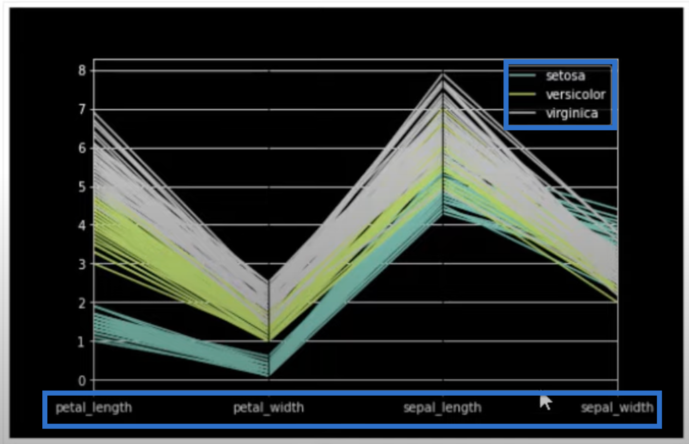
Parallel Coordinate Plots In Python: Sample 2
Our second plot is an iris dataset showing petal_length, petal_width, sepal_length, and sepal_width. It has a little bit more style in comparison to the first graph.
This dataset was created with Python code.
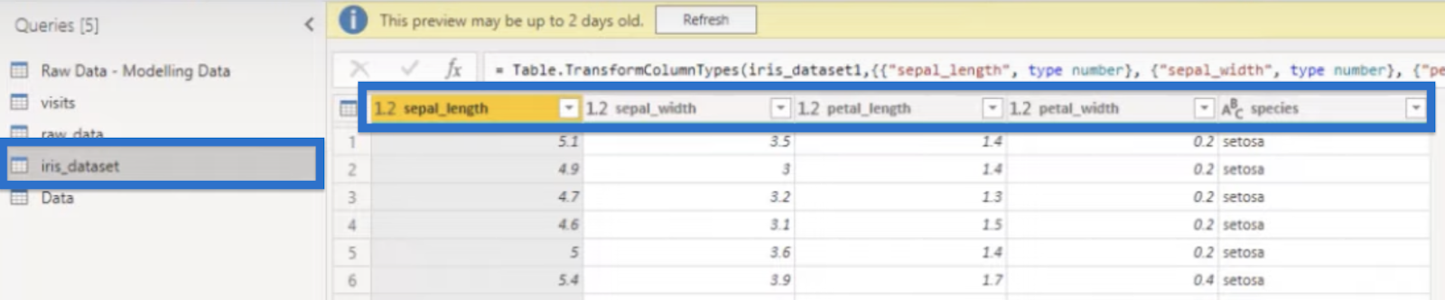
To view our data, click Transform data and go to the iris_dataset.

The dataset contains columns for the dimensions—sepal length, sepal width, petal length, and petal width. It also has a column for the species type.
The Dataset Python Code
Our data was brought in easily using Python code. Go to Source to show the Python script.
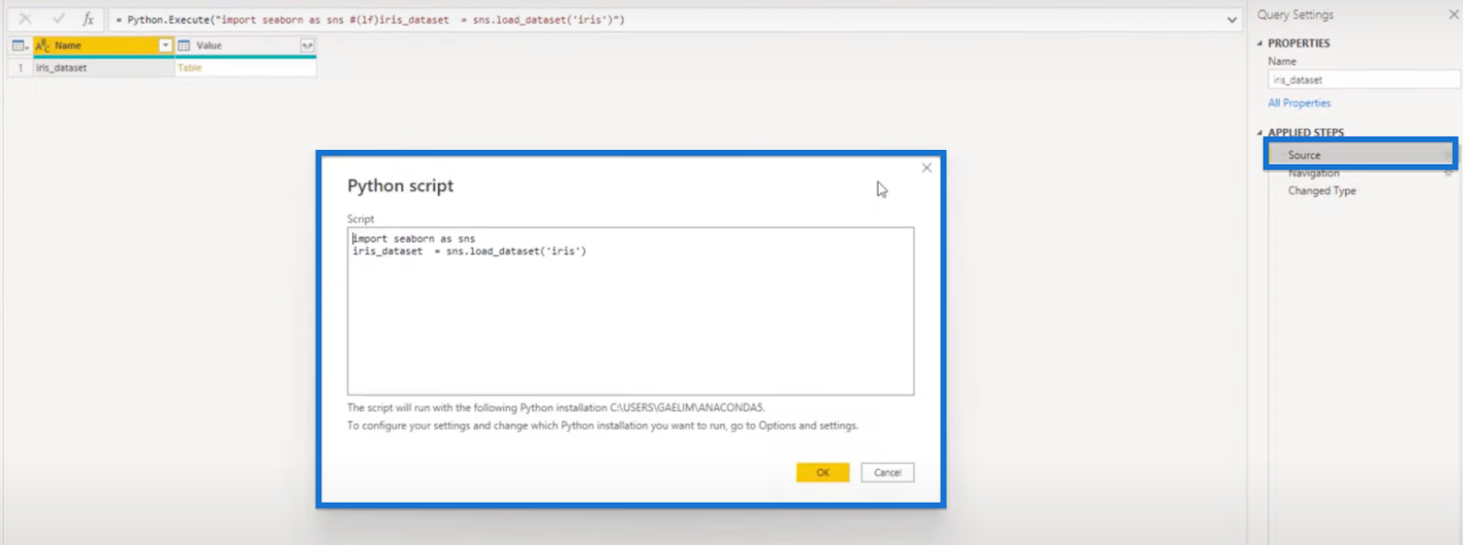
Our Python code has only two lines. In the first line, we imported seaborn and saved it as variable sns. We named our dataset as iris_dataset and used the sns variable to load the dataset using the sns.load_dataset(‘iris’) function.

Click OK to get the data we’ve seen above. Navigate through the data, and once done, we can close the dataset by going to Close & Apply > Close.

Styling Plots In Python
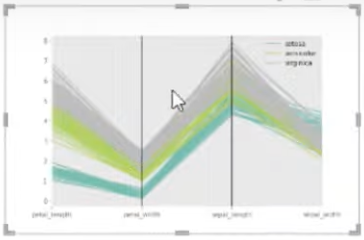
To open the Python script editor for our more stylized graph, click our second plot.
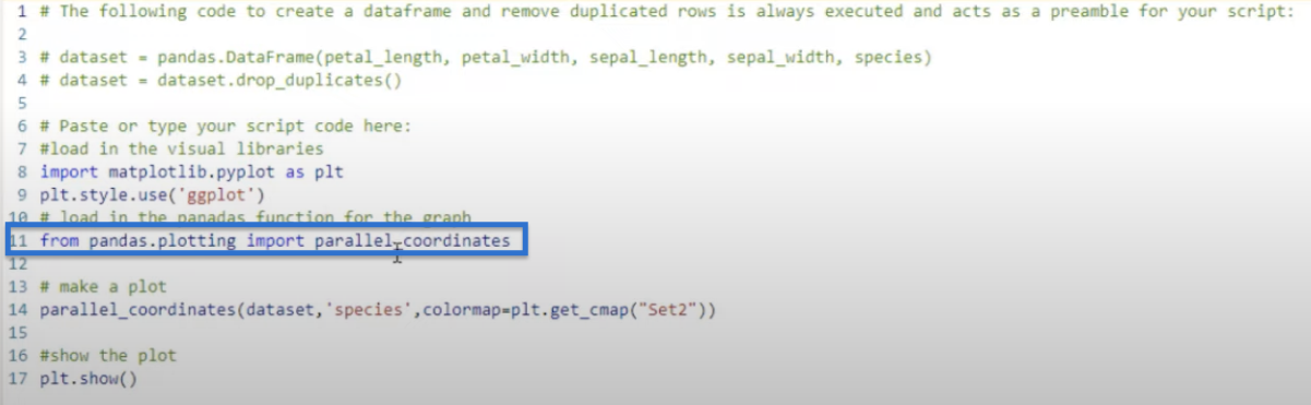
We start by importing matplotlib.pyplot as plt.

Then, we use the function plt.style.use (‘dark_background’) to style the visual.

We can easily customize the background based on our preferred style using matplotlib’s Style sheet reference. In our case, we used a dark background.

Let’s also try using ggplot, which is a common style used.

If we run it, it will give us a visual that looks like this.
Then, load the pandas function for the graph by importing parallel_coordinates from pandas.plotting.
To make the plot, we bring in the dataset and set our species as the class.

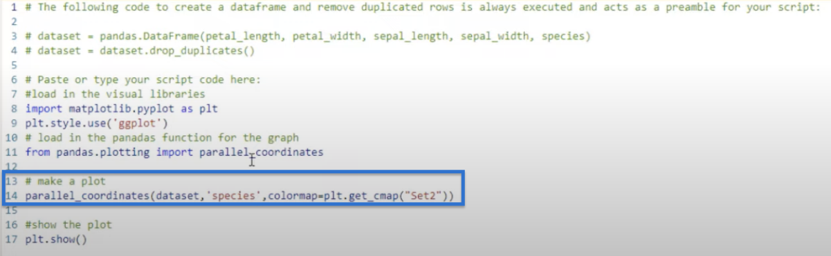
Compared to our first plot, we add an additional parameter which is the colormap to get different colors. Pass that in using the matplotlib variable, plt.get_cmap.

There are a lot of matplotlib color variables to choose from in the matplotlib’s Colormap reference.

For example, we are currently using Set 2 from Qualitative colormaps but we can also change that to other colors, such as hsv from Cyclic colormaps.

Click run to get a plot that looks like this.

Hsv doesn’t look very good on our data, but we can play around until we find the most suitable colormap for our plot.
***** Related Links *****
Python Correlation: Guide In Creating Visuals
Datasets In Pandas With ProfileReport() | Python In Power BI
Seaborn Function In Python To Visualize A Variable’s Distribution
Conclusion
In this tutorial, we have covered the basics of creating parallel coordinate plots in Python. We have gone through the process of preparing the data, creating the plot, and customizing the plot for better readability.
Parallel coordinate plots are a powerful tool for visualizing high-dimensional data and can be used in a variety of fields including finance, engineering, and machine learning. Now that we know how to create parallel coordinate plots in Python, we can start using them to better understand and visualize our own data.
All the best,
Gaelim Holland


")